Tensors in PyTorch

Tensors are one of the most fundamental concepts in Artificial Intelligence (AI), Machine Learning (ML), and Deep Learning. Every popular deep learning framework such as PyTorch, TensorFlow, and JAX uses tensors to store and process data efficiently.

If you’ve ever worked with arrays in Python using NumPy, you already understand the basic idea. A tensor is simply an extension of an array that can represent data in any number of dimensions.

In this guide, we’ll understand tensors from scratch with real-world examples used in deep learning.

What is a Tensor? #

A tensor is a specialized multi-dimensional array designed for efficient mathematical computations.

In simple words: What an array does in one dimension, a tensor does in multiple dimensions.

A tensor is a generalized form of:

• Scalar (0D)
• Vector (1D)
• Matrix (2D)
• Higher-dimensional arrays (3D, 4D, 5D, and beyond)

Because deep learning models perform millions of mathematical operations, tensors are optimized to make these computations fast on CPUs, GPUs, and TPUs.

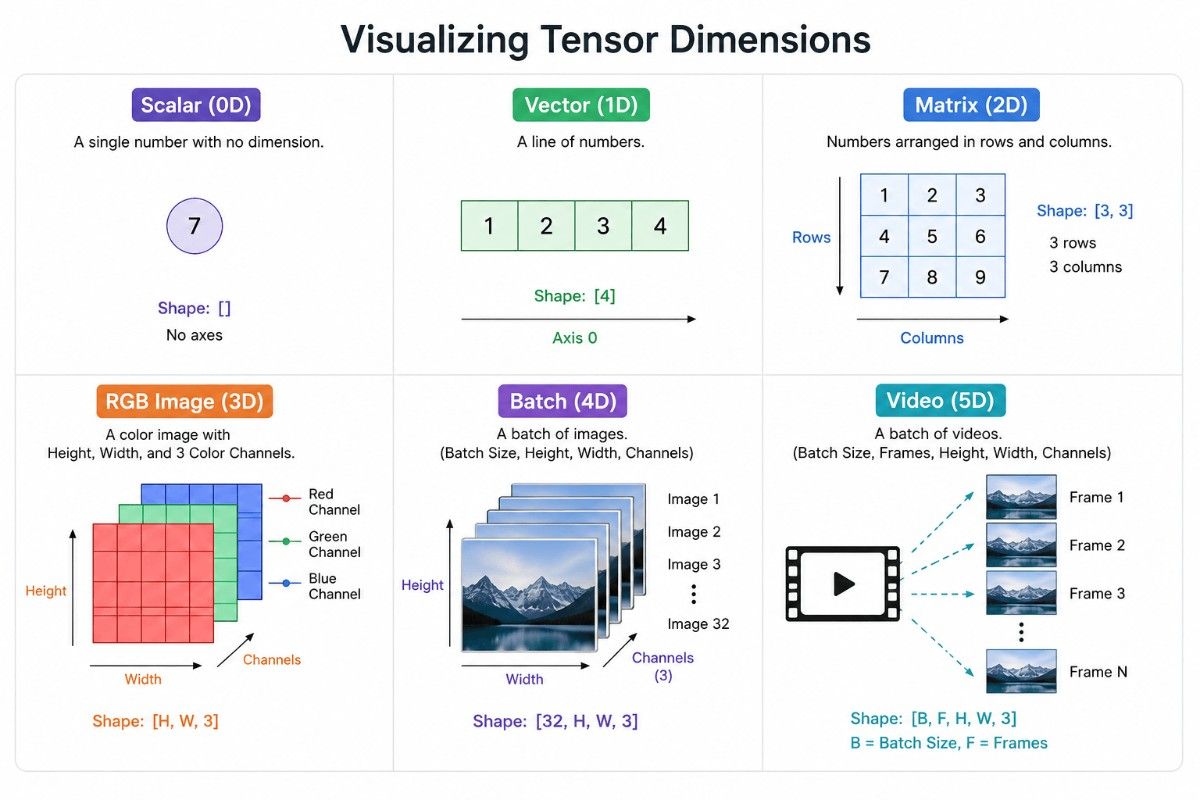
Understanding Tensor Dimensions #

The dimension (or rank) of a tensor tells us how many directions (axes) the data extends.

Each new dimension adds another level of organization.

For example:

• One direction → Vector
• Two directions → Matrix
• Three directions → Cube-like structure
• More dimensions → Collections of complex data

Understanding tensor dimensions is essential because almost every deep learning operation involves manipulating tensor shapes.

0-Dimensional Tensor (Scalar) #

A 0D tensor, also called a scalar, contains only a single value.

It has no direction and no axis.

Ex: 3.14

---

Deep Learning Example #

During neural network training, the model predicts an output.

The loss function calculates how far the prediction is from the actual value.

The output is always a single number, such as:

Loss = 0.234

This loss value is a 0D tensor.

1-Dimensional Tensor (Vector) #

A 1D tensor extends in one direction.

It is similar to a Python list or NumPy array.

Example #

[2, 5, 7, 10]

Shape:

[4]

because it contains four elements.

---

Deep Learning Example #

One of the most common applications is Word Embeddings.

Natural language cannot be directly understood by computers.

Instead, each word is converted into numbers.

For example,

"Hello"

may become

[0.21, -0.74, 0.56, 1.12]

Each value represents some learned characteristic of the word.

Popular embedding models include:

• Word2Vec
• GloVe
• FastText

Modern Transformer models also generate embedding vectors.

---

2-Dimensional Tensor (Matrix) #

A 2D tensor consists of rows and columns.

It looks exactly like a spreadsheet.

Example #

[
 [1, 2, 3],
 [4, 5, 6]
]

Shape:

[2, 3]

Meaning:

• 2 rows
• 3 columns

---

Deep Learning Example #

Grayscale images are stored as 2D tensors.

Each pixel contains one intensity value.

Example:

28 × 28

The famous MNIST handwritten digit dataset uses grayscale images.

Its tensor shape is:

[28, 28]

Each value ranges from:

0 → Black

255 → White

---

3-Dimensional Tensor #

A 3D tensor extends in three directions.

One extra dimension is added to store multiple matrices.

---

Deep Learning Example #

A color image contains three separate channels:

• Red
• Green
• Blue

Each channel is itself a grayscale image.

Together they form an RGB image.

Shape:

[Height, Width, Channels]

Example:

[256, 256, 3]

Meaning:

• Height = 256 pixels
• Width = 256 pixels
• RGB channels = 3

---

4-Dimensional Tensor #

Instead of training on one image at a time, deep learning models train on batches.

A batch is simply multiple images processed together.

Shape:

[Batch Size, Height, Width, Channels]

Example:

[32, 128, 128, 3]

Meaning:

• 32 images
• Each image is 128 × 128
• RGB channels

---

Why Use Batches? #

Training one image at a time is inefficient.

Batch processing provides:

• Faster GPU computation
• Better memory utilization
• Stable gradient updates
• Reduced training time

This is why almost every neural network uses mini-batches during training.

---

5-Dimensional Tensor #

Videos are collections of images displayed rapidly.

Each image is called a frame.

A video therefore adds another dimension called Frames.

Shape:

[Batch Size, Frames, Height, Width, Channels]

Example:

[10, 16, 64, 64, 3]

Meaning:

• 10 video clips
• 16 frames in each clip
• Frame size = 64 × 64
• RGB channels

---

Understanding Video as Tensors #

Imagine a moving football.

Frame 1:

Ball at Position A

Frame 2:

Ball moving

Frame 3:

Ball at Position B

When these frames are displayed quickly (typically 24–60 frames per second), our eyes perceive smooth motion.

Deep learning models process the entire sequence as a 5D tensor.

Applications include:

• Action recognition
• Video classification
• Object tracking
• Surveillance systems
• Autonomous driving

---

Why Are Tensors Important? #

Tensors are the foundation of deep learning because they provide:

1. Flexibility #

They can represent simple numbers or highly complex datasets.

2. Computational Efficiency #

Tensor operations are heavily optimized for GPUs and TPUs.

3. Scalability #

From one number to millions of values, tensors scale effortlessly.

4. Mathematical Operations #

Deep learning consists mainly of tensor operations such as:

• Addition
• Multiplication
• Matrix multiplication
• Transpose
• Reshaping
• Broadcasting

---

Key Takeaways #

• A tensor is a multi-dimensional array optimized for mathematical computation.
• Scalars, vectors, and matrices are all special cases of tensors.
• The number of dimensions determines how data is organized.
• Images, text, audio, and videos are all represented as tensors in deep learning.
• Modern frameworks like PyTorch and TensorFlow perform almost every operation using tensors.
• Understanding tensor dimensions and shapes is essential before learning neural networks, convolutional neural networks (CNNs), transformers, or large language models (LLMs).

Creating a Tensor #

import torch

# Using empty
a = torch.empty(2,3)
print(a)
# Output:
# tensor([[ 1.4013e-45,  0.0000e+00,  2.8026e-45],
#         [ 4.2039e-45,  5.6052e-45,  7.0065e-45]])
# (Values may differ because memory is uninitialized.)

# Check type
print(type(a))
# Output:
# <class 'torch.Tensor'>

# Using zeros
print(torch.zeros(2,3))
# Output:
# tensor([[0., 0., 0.],
#         [0., 0., 0.]])

# Using ones
print(torch.ones(2,3))
# Output:
# tensor([[1., 1., 1.],
#         [1., 1., 1.]])

# Using rand
print(torch.rand(2,3))
# Output:
# tensor([[0.2961, 0.5166, 0.2517],
#         [0.6886, 0.0740, 0.8665]])
# (Values are random and will be different each time.)

# Another random tensor
print(torch.rand(2,3))
# Output:
# tensor([[0.1366, 0.1025, 0.1841],
#         [0.7264, 0.3153, 0.6871]])
# (Values are random.)

# Using manual_seed
torch.manual_seed(100)
print(torch.rand(2,3))
# Output:
# tensor([[0.1117, 0.8158, 0.2626],
#         [0.4839, 0.6765, 0.7539]])

# Same seed gives the same output
torch.manual_seed(100)
print(torch.rand(2,3))
# Output:
# tensor([[0.1117, 0.8158, 0.2626],
#         [0.4839, 0.6765, 0.7539]])

# Using tensor
print(torch.tensor([[1,2,3],[4,5,6]]))
# Output:
# tensor([[1, 2, 3],
#         [4, 5, 6]])

# Using arange
print("using arange ->", torch.arange(0,10,2))
# Output:
# using arange -> tensor([0, 2, 4, 6, 8])

# Using linspace
print("using linspace ->", torch.linspace(0,10,10))
# Output:
# using linspace -> tensor([ 0.0000,  1.1111,  2.2222,  3.3333,  4.4444,
#                            5.5556,  6.6667,  7.7778,  8.8889, 10.0000])

# Using eye
print("using eye ->", torch.eye(5))
# Output:
# using eye -> tensor([[1., 0., 0., 0., 0.],
#                      [0., 1., 0., 0., 0.],
#                      [0., 0., 1., 0., 0.],
#                      [0., 0., 0., 1., 0.],
#                      [0., 0., 0., 0., 1.]])

# Using full
print("using full ->", torch.full((3, 3), 5))
# Output:
# using full -> tensor([[5, 5, 5],
#                       [5, 5, 5],
#                       [5, 5, 5]])

Tensor Shapes #

import torch

# Create a tensor
x = torch.tensor([[1, 2, 3],
                  [4, 5, 6]])
print(x)
# Output:
# tensor([[1, 2, 3],
#         [4, 5, 6]])

# Check tensor shape
print("Shape of x:", x.shape)
# Output:
# Shape of x: torch.Size([2, 3])

# Create an empty tensor with the same shape
print("Empty Like:\n", torch.empty_like(x))
# Output:
# Empty Like:
# tensor([[     0, 32767,     0],
#         [     0,     0,     0]])
# (Values may differ because the tensor is uninitialized.)

# Create a zero tensor with the same shape
print("Zeros Like:\n", torch.zeros_like(x))
# Output:
# Zeros Like:
# tensor([[0, 0, 0],
#         [0, 0, 0]])

# Create a tensor filled with ones having the same shape
print("Ones Like:\n", torch.ones_like(x))
# Output:
# Ones Like:
# tensor([[1, 1, 1],
#         [1, 1, 1]])

# Create a random tensor with the same shape
print("Random Like:\n", torch.rand_like(x, dtype=torch.float))
# Output:
# Random Like:
# tensor([[0.2961, 0.5166, 0.2517],
#         [0.6886, 0.0740, 0.8665]])
# (Values are random and will be different each time.)

Tensor Data Types #

# Create tensors with different data types

# Integer tensor
x = torch.tensor([1, 2, 3])
print(x.dtype)
# Output: torch.int64

# Float tensor
y = torch.tensor([1.5, 2.5, 3.5])
print(y.dtype)
# Output: torch.float32

# Boolean tensor
z = torch.tensor([True, False, True])
print(z.dtype)
# Output: torch.bool

# Create tensor with a specific data type
a = torch.tensor([1, 2, 3], dtype=torch.float32)
print(a.dtype)
# Output: torch.float32

b = torch.tensor([1, 2, 3], dtype=torch.int32)
print(b.dtype)
# Output: torch.int32

# Change data type using type()
c = a.type(torch.int64)
print(c.dtype)
# Output: torch.int64

# Change data type using to()
d = b.to(torch.float64)
print(d.dtype)
# Output: torch.float64

Data Type	Description	Example
torch.int8	8-bit signed integer	[-128, 127]
torch.int16	16-bit signed integer	Small integers
torch.int32	32-bit signed integer	Integer computations
torch.int64	64-bit signed integer (default integer type)	Labels, indices
torch.float16	16-bit floating point	Faster GPU training
torch.float32	32-bit floating point (default float type)	Neural network computations
torch.float64	64-bit floating point	High-precision calculations
torch.bool	Boolean values	True, False

Mathematical Operations. #

import torch

# Create two tensors
a = torch.tensor([2, 4, 6])
b = torch.tensor([1, 3, 5])

# Addition
print(a + b)
# Output: tensor([3, 7, 11])

# Subtraction
print(a - b)
# Output: tensor([1, 1, 1])

# Multiplication (Element-wise)
print(a * b)
# Output: tensor([ 2, 12, 30])

# Division
print(a / b)
# Output: tensor([2.0000, 1.3333, 1.2000])

# Exponentiation
print(a ** 2)
# Output: tensor([ 4, 16, 36])

# Square Root
print(torch.sqrt(a.float()))
# Output: tensor([1.4142, 2.0000, 2.4495])

# Sum of all elements
print(torch.sum(a))
# Output: tensor(12)

# Mean
print(torch.mean(a.float()))
# Output: tensor(4.)

# Maximum value
print(torch.max(a))
# Output: tensor(6)

# Minimum value
print(torch.min(a))
# Output: tensor(2)

# Matrix Multiplication
x = torch.tensor([[1, 2],
                  [3, 4]])

y = torch.tensor([[5, 6],
                  [7, 8]])

print(torch.matmul(x, y))
# Output:
# tensor([[19, 22],
#         [43, 50]])

Reduction operation #

Reduction operations reduce multiple tensor elements into a single value (or fewer values) by applying operations such as sum, mean, maximum, or minimum. These operations are commonly used in deep learning to calculate statistics, evaluate model performance, and compute loss values.

import torch

# Create a tensor
x = torch.tensor([[1, 2, 3],
                  [4, 5, 6]], dtype=torch.float32)

# Sum of all elements
print(torch.sum(x))
# Output: tensor(21.)

# Mean of all elements
print(torch.mean(x))
# Output: tensor(3.5000)

# Maximum value
print(torch.max(x))
# Output: tensor(6.)

# Minimum value
print(torch.min(x))
# Output: tensor(1.)

# Row-wise Sum
print(torch.sum(x, dim=1))
# Output: tensor([ 6., 15.])

# Column-wise Sum
print(torch.sum(x, dim=0))
# Output: tensor([5., 7., 9.])

# Row-wise Mean
print(torch.mean(x, dim=1))
# Output: tensor([2., 5.])

# Column-wise Mean
print(torch.mean(x, dim=0))
# Output: tensor([2.5000, 3.5000, 4.5000])

# Index of Maximum Value
print(torch.argmax(x))
# Output: tensor(5)

# Index of Minimum Value
print(torch.argmin(x))
# Output: tensor(0)

Matrix operations #

Matrix operations are fundamental in deep learning because they are used to perform computations in neural networks. PyTorch provides several built-in functions for matrix multiplication, transpose, and finding the inverse of a matrix. Unlike element-wise operations, matrix operations follow the rules of linear algebra.

import torch

# Create two matrices
A = torch.tensor([[1, 2],
                  [3, 4]], dtype=torch.float32)

B = torch.tensor([[5, 6],
                  [7, 8]], dtype=torch.float32)

# Matrix Multiplication
print(torch.matmul(A, B))
# Output:
# tensor([[19., 22.],
#         [43., 50.]])

# Matrix Multiplication using @ operator
print(A @ B)
# Output:
# tensor([[19., 22.],
#         [43., 50.]])

# Transpose of a matrix
print(A.T)
# Output:
# tensor([[1., 3.],
#         [2., 4.]])

# Matrix Inverse
print(torch.inverse(A))
# Output:
# tensor([[-2.0000,  1.0000],
#         [ 1.5000, -0.5000]])

# Matrix Determinant
print(torch.det(A))
# Output:
# tensor(-2.)

# Matrix Trace
print(torch.trace(A))
# Output:
# tensor(5.)

# Matrix Rank
print(torch.linalg.matrix_rank(A))
# Output:
# tensor(2)

Comparison operations #

Comparison operations are used to compare the values of two tensors element by element. Instead of returning numerical values, these operations return Boolean tensors, where True indicates that the comparison is satisfied and False indicates that it is is not. These operations are commonly used in deep learning for filtering data, creating masks, and applying conditional logic.

import torch

# Create two tensors
a = torch.tensor([1, 2, 3, 4])
b = torch.tensor([2, 2, 1, 4])

# Equal
print(torch.eq(a, b))
# Output: tensor([False,  True, False,  True])

# Not Equal
print(torch.ne(a, b))
# Output: tensor([ True, False,  True, False])

# Greater Than
print(torch.gt(a, b))
# Output: tensor([False, False,  True, False])

# Greater Than or Equal
print(torch.ge(a, b))
# Output: tensor([False,  True,  True,  True])

# Less Than
print(torch.lt(a, b))
# Output: tensor([ True, False, False, False])

# Less Than or Equal
print(torch.le(a, b))
# Output: tensor([ True,  True, False,  True])

# Check if all elements are equal
print(torch.equal(a, b))
# Output: False

Special Functions #

Special functions perform common mathematical operations on tensors such as absolute value, rounding, exponentials, logarithms, and trigonometric calculations. These functions are widely used in deep learning, scientific computing, and data preprocessing.

import torch

# Create a tensor
x = torch.tensor([-2.5, -1.2, 0.0, 1.8, 3.6])

# Absolute value
print(torch.abs(x))
# Output: tensor([2.5000, 1.2000, 0.0000, 1.8000, 3.6000])

# Round to nearest integer
print(torch.round(x))
# Output: tensor([-2., -1.,  0.,  2.,  4.])

# Floor (round down)
print(torch.floor(x))
# Output: tensor([-3., -2.,  0.,  1.,  3.])

# Ceil (round up)
print(torch.ceil(x))
# Output: tensor([-2., -1.,  0.,  2.,  4.])

# Clamp values between 0 and 2
print(torch.clamp(x, min=0, max=2))
# Output: tensor([0.0000, 0.0000, 0.0000, 1.8000, 2.0000])

# Exponential
print(torch.exp(torch.tensor([1., 2.])))
# Output: tensor([2.7183, 7.3891])

# Natural Logarithm
print(torch.log(torch.tensor([1., 2., 4.])))
# Output: tensor([0.0000, 0.6931, 1.3863])

# Square Root
print(torch.sqrt(torch.tensor([4., 9., 16.])))
# Output: tensor([2., 3., 4.])

# Sine
print(torch.sin(torch.tensor([0., 1.5708])))
# Output: tensor([0.0000, 1.0000])

# Cosine
print(torch.cos(torch.tensor([0., 1.5708])))
# Output: tensor([ 1.0000e+00, -3.6199e-06])

Inplace Operations #

In-place operations modify the original tensor directly without creating a new tensor. In PyTorch, most in-place operations have an underscore (_) at the end of the function name, such as add_(), mul_(), and zero_(). These operations are memory-efficient because they update the existing tensor instead of allocating new memory. However, they should be used carefully during deep learning model training, as they can interfere with PyTorch’s automatic differentiation (autograd).

import torch

# Create a tensor
x = torch.tensor([1., 2., 3.])
print("Original Tensor:", x)
# Output: tensor([1., 2., 3.])

# In-place Addition
x.add_(5)
print("After add_():", x)
# Output: tensor([6., 7., 8.])

# In-place Multiplication
x.mul_(2)
print("After mul_():", x)
# Output: tensor([12., 14., 16.])

# In-place Subtraction
x.sub_(2)
print("After sub_():", x)
# Output: tensor([10., 12., 14.])

# In-place Division
x.div_(2)
print("After div_():", x)
# Output: tensor([5., 6., 7.])

# In-place Fill
x.fill_(1)
print("After fill_():", x)
# Output: tensor([1., 1., 1.])

# In-place Zero
x.zero_()
print("After zero_():", x)
# Output: tensor([0., 0., 0.])

Copying a Tensor #

When working with tensors in PyTorch, it is important to understand the difference between assigning a tensor and copying a tensor. Assigning one tensor to another variable does not create a new tensor; instead, both variables refer to the same memory location. To create an independent copy, PyTorch provides the clone() method. This is especially useful in deep learning when you want to preserve the original tensor while modifying its copy.

import torch

# Create a tensor
a = torch.tensor([1, 2, 3])
print("Original Tensor:", a)
# Output: tensor([1, 2, 3])

# Assignment (No Copy)
b = a
print("Tensor b:", b)
# Output: tensor([1, 2, 3])

# Modify b
b[0] = 100
print("After modifying b:")
print("a =", a)
# Output: tensor([100,   2,   3])
print("b =", b)
# Output: tensor([100,   2,   3])

# Create an independent copy
c = a.clone()
print("Tensor c:", c)
# Output: tensor([100,   2,   3])

# Modify c
c[1] = 200
print("After modifying c:")
print("a =", a)
# Output: tensor([100,   2,   3])
print("c =", c)
# Output: tensor([100, 200,   3])

# Check memory addresses
print("ID of a:", id(a))
# Output: (Memory address of a)

print("ID of b:", id(b))
# Output: Same memory address as a

print("ID of c:", id(c))
# Output: Different memory address

Tensors in PyTorch #