Welcome to the start of your journey into Machine Learning (ML). For many, ML feels like a “black box” a mysterious process where data goes in and magic comes out. As a Senior Educator, my goal is to peel back those layers and show you that ML is not magic; it is a structured, logical evolution of how we solve problems using computers. Think of it this way: we are moving from being “Dictators” who tell computers exactly what to do, to “Mentors” who show computers how to learn from examples.
1. The Great Paradigm Shift: From Rules to Patterns #
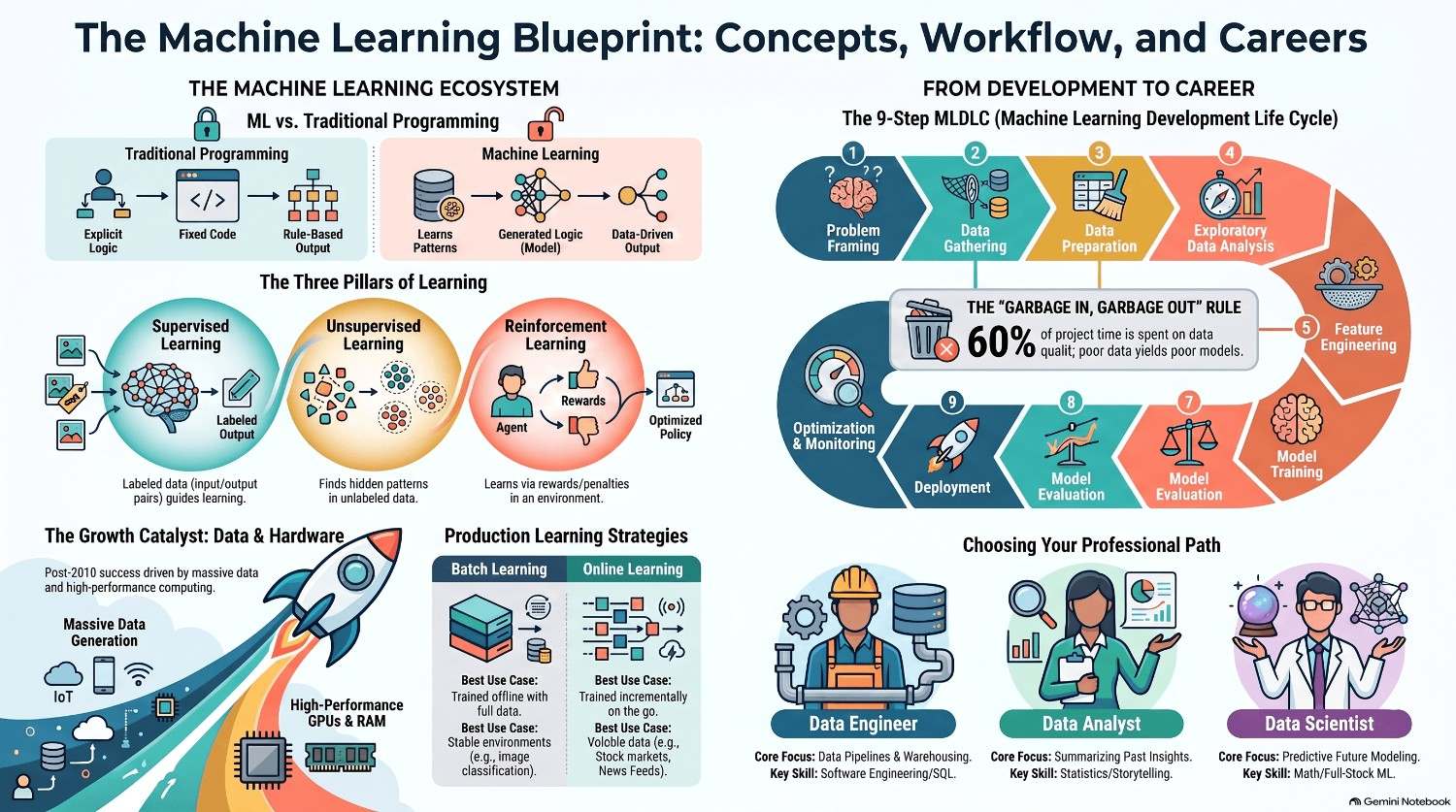
To understand Machine Learning, you must first understand how it differs from traditional software development. In conventional programming, humans are the “brains” behind every decision. In ML, the computer learns to find the “logic” itself.
Conventional Programming vs. Machine Learning
| Feature | Conventional Programming | Machine Learning |
|---|---|---|
| Input Components | Logic (Code) + Data | Data + Output (Answers) |
| The Result | Output (The Answer) | Logic (The Model/Rules) |
| Human Role | Creating explicit “if-then” rules | Providing high-quality examples |
| Adaptability | Rigid; requires manual updates | Fluid; evolves with new data |
Illustrative Examples of the Shift
- Adding Numbers: In conventional coding, a function like
sum(a, b)has strict functional limits. If you suddenly need to add three or ten numbers, the code physically cannot handle it without a human developer rewriting the logic. In ML, you provide an Excel file with thousands of rows of various numbers and their sums. The algorithm recognizes the “operator” essence of addition. It learns the pattern, allowing it to scale to any number of inputs without a single line of new code. - The Email Spam Cat-and-Mouse Game: Hardcoding spam filters using keywords like “discount” is a losing battle. Once spammers switch to “d1scount,” a hardcoded rule fails. ML stays ahead of this game by evolving with the data; it recognizes the shifting patterns of spam automatically, requiring no manual intervention to catch the new variations.
- The Fuzzy Logic of Dogs: How do you program a computer to recognize a dog? With thousands of breeds, sizes, and lighting conditions, you could never write enough “if-then” rules to capture them all. This is the “Fuzzy Logic” problem—rules are too brittle for the messiness of the real world. ML solves this by “learning like a human”—we show the system thousands of tagged photos until it identifies the underlying “dog-ness” in an image.
While we’ve seen how ML changes the problem-solving process, we must understand where it sits within the broader landscape of technology.
2. The Core Hierarchy: AI vs. ML vs. DL #
To visualize the relationship between these fields, imagine a Venn Diagram with three nested circles. The outermost circle is Artificial Intelligence (AI), the broad universe of “smart” machines. Inside that sits Machine Learning (ML), a specific solar system of algorithms. At the very center, the core, is Deep Learning (DL).
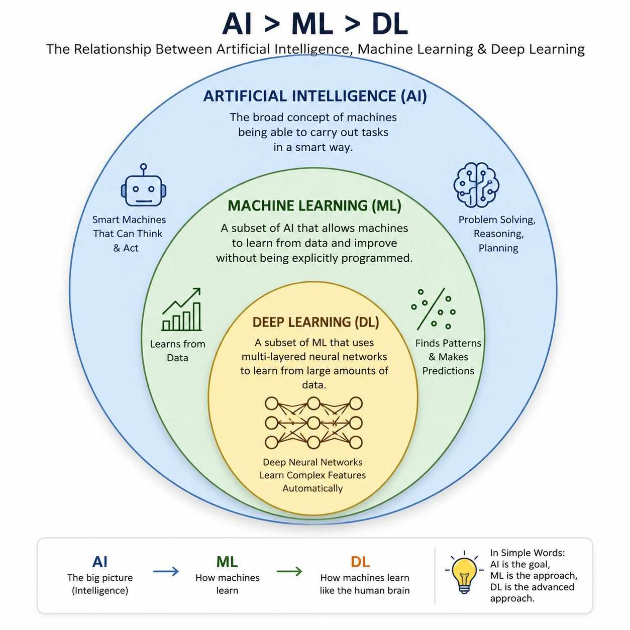
- Artificial Intelligence (AI): The broad goal of giving machines “intelligence.” Modern AI focuses almost entirely on Pattern Recognition. It is important to note that elements of human intelligence—such as true creativity, imagination, and emotional intelligence—remain currently out of reach for these systems.
- Expert Systems (Symbolic AI): An early branch of AI that used hardcoded “knowledge bases.” While successful at logical games like Chess, they failed at “fuzzy” problems like voice or image recognition because they couldn’t handle real-world variations.
- Machine Learning (ML): A branch of computer science using statistical techniques to find patterns in data without explicit programming.
- Deep Learning (DL): A subset of ML inspired by biological neurons. Its “superpower” is Automatic Feature Extraction. In classical ML, a human must manually define features (e.g., “look at pointed ears”). In DL, the system identifies edges, shapes, and textures itself, making it far superior for “fuzzy” data like images or raw text.
The “So What?”: Why Classical ML Still Reigns You might wonder why we don’t use Deep Learning for everything. Here is a reality check:
- The 90% Rule: While tech giants like Google deal with “Big Data,” 90% of the world’s data—especially in banking, insurance, and sports analytics—is actually “Small Data.”
- Efficiency: For these smaller datasets, classical ML is faster, cheaper, and often more accurate than DL.
- Practicality: In most corporate environments, a well-tuned classical ML model is more vital than a complex neural network.
Once we understand the hierarchy, we can categorize how these machines actually learn.
3. The Multi-Dimensional Taxonomy of Machine Learning #
Machine Learning is categorized by the “amount of supervision” the system receives.
- Supervised Learning: The system is trained on a labeled dataset (Input + Output).
- Regression: Predicting a numerical value (e.g., house prices).
- Classification: Predicting a category (e.g., “Spam” vs. “Not Spam”).
- Unsupervised Learning: The system finds hidden structures in unlabeled data.
- Clustering: Grouping students by similar IQ and GPA.
- Dimensionality Reduction: Think of the MNIST dataset of handwritten digits. Each image has 784 pixels (dimensions), which is impossible for humans to visualize. Techniques like t-SNE squash these 784 dimensions into a 3D “cloud” where we can actually see clusters of “6s” or “4s” grouped together.
- Anomaly Detection: Finding the “green point” (the outlier) in a sea of red points, such as spotting credit card fraud.
- Association Rule Learning: Finding hidden correlations, such as the famous Walmart study where data revealed that customers buying diapers were also likely to buy beer.
- Semi-Supervised Learning: This is used when labeling is expensive. In Google Photos, the system uses unsupervised clustering to group similar faces. It then asks a human to label just one photo. That single label is propagated to the entire cluster, saving hours of manual work.
- Reinforcement Learning: An Agent learns by interacting with an Environment to maximize a Reward. This is how AlphaGo defeated Lee Sedol—by playing millions of games against itself and reinforcing winning strategies.
Knowing the category of learning is only the beginning; building a product requires a rigorous engineering roadmap.
4. The 9-Step Machine Learning Development Life Cycle (MLDLC) #
Here is where most students get tripped up: they think ML is just “running a model.” In reality, it is a 9-step professional process:
- Problem Framing: Translating business goals (e.g., Netflix churn reduction) into a mathematical problem.
- Data Gathering: Sourcing data from APIs, Web Scraping, or Data Warehouses (ETL).
- Pre-processing: The “cleaning” phase—removing duplicates, scaling, and handling missing values.
- EDA (Exploratory Data Analysis): This is the “Sharpening the axe” phase. Recall the analogy: if you have 6 hours to cut a tree, spend 4 hours sharpening the axe. By performing Univariate and Bivariate analysis, the actual modeling becomes effortless.
- Feature Engineering & Selection: Creating new columns (like BMI from height/weight) and dropping irrelevant ones.
- Model Training: Testing a “Family of Models” to see which algorithm fits the pattern best.
- Evaluation: Using metrics like Accuracy or Mean Squared Error.
- Deployment: Converting models to APIs on platforms like AWS, GCP, or Heroku.
- Testing & Optimization: Using A/B Testing and monitoring for Model Rot—the natural decline in performance as real-world data changes.
While this roadmap is clear, the path is fraught with the messy realities of the industry.
5. Reality Check: Messy Realities and Challenges #
- The Data Quality Burden: Expect to spend 60-80% of your project time cleaning “garbage” data.
- Representative Sampling (Noise vs. Bias): Using the T20 World Cup survey example:
- Sampling Noise: You only survey one location (India) for a global event. You don’t have enough data to be accurate.
- Sampling Bias: You survey a large group globally, but they are all Indians. Your data is prejudiced and qualitatively wrong.
- The Overfitting Villain: This is “memorization” instead of “generalization.” If you see a ₹1200 movie ticket in Gurgaon and conclude “Everything in Gurgaon is expensive,” you have overfitted your model to a single experience.
- Software Integration: Python models often struggle to work seamlessly in Java or JavaScript environments.
- The Cloud Cost Trap: High-scale deployment can lead to massive, unexpected bills if not optimized for efficiency.
Navigating these challenges requires choosing the right career path and skill set.
6. Navigating Careers in the Data Space #
| Role | Core Mission | Primary Skillset |
|---|---|---|
| Data Engineer | The “Plumbing”: Moving data from A to B. | SQL, Big Data, Spark, ETL. |
| Data Analyst | The “History”: Explaining the past. | Stats, SQL, Visualization, Storytelling. |
| Data Scientist | The “Full Stack”: Modeling the future. | ML, Stats, Business Acumen. |
| ML Engineer | The “Bridge”: Deploying to production. | Software Engineering, MLOps, Deployment. |
The Master Teacher’s 3-Step Action Plan
- Memorize the 9 steps of the MLDLC: They are your North Star.
- Build an end-to-end product: Don’t just stop at an accuracy score on your laptop; deploy it as an API.
- Check job boards: Look for the current demand for specific tools like Spark, AWS, or MLOps to guide your study.
Machine Learning is a rising curve. By focusing on the engineering process rather than just the “magic,” you are positioning yourself at the forefront of the next technological revolution.
Batch Learning vs. Online Learning #
The primary difference between Batch Learning and Online Learning is how a machine learning model is trained and updated once it is sent to a live production environment.
| Feature | Batch Learning (Offline Learning) | Online Learning (Incremental Learning) |
|---|---|---|
| Training Method | Trains on the entire dataset all at once. No incremental training is allowed. | Trains incrementally using small sequential chunks of data called “mini-batches”. |
| Location of Training | Typically done offline on a data scientist’s development machine because training is slow and computationally expensive. | Done directly on the live production server on the fly. |
| How Updates Happen | To update, you must pull down the model, merge the old data with new data, retrain the entire dataset from scratch, and redeploy. | The model dynamically learns and improves its performance continuously as live data streams in. |
| Production Speed | Highly stable and easy to implement in production, but update latency is high (typically 24-hour, weekly, or monthly cycles). | Extremely fast training (e.g., using algorithms that can train on a single data point in 0.04 seconds). |
Crucial Concepts in Online Learning
- Out-of-Core Learning: If you have a massive dataset (e.g., 50 GB) but your machine only has 8 GB of RAM, you cannot load the data all at once for batch training. Out-of-core learning solves this by splitting the massive dataset into smaller chunks and training the model sequentially offline using online learning techniques.
- Concept Drift: In volatile markets (like stock exchanges or e-commerce), the patterns in data change rapidly over time. While batch learning models easily become obsolete (such as a spam filter decaying over a year as spammers adapt), online learning models dynamically adjust on the fly to combat concept drift.
- Learning Rate: Setting the correct learning rate is the most difficult part of online learning. If set too high, the model will learn new trends quickly but immediately forget old patterns; if set too low, it will learn too slowly.
- The Risk of Data Poisoning: If someone manipulates or sends malicious data to your live server, an online model will learn from this bad data and its behavior can quickly become biased or broken. This makes online learning highly risky, requiring active anomaly detection monitoring and instant rollback systems to restore the model to a previous safe state.
- Implementation Tools: In Scikit-Learn, models like SGDRegressor support online learning via the
.partial_fit()method instead of.fit(). There are also dedicated streaming machine learning libraries like River (a merger of Creme and scikit-multiflow) and Vowpal Wabbit.
Instance-Based Learning vs. Model-Based Learning #
This taxonomy is based on how a machine learning model learns and generalizes to new data.
1. Instance-Based Learning (“The Memorizer”)
Instance-based learning is akin to rote memorization.
- How it Works: The algorithm does not perform any actual math or pattern extraction during the training phase. Instead, it simply stores the entire training dataset in memory.
- The Lazy Learner: It is called a “lazy learner” because it sits completely idle during training. It only starts working when a new, unseen query point is introduced.
- Making Predictions: To predict, it calculates the mathematical distance (similarity) between the new query point and all the stored training instances. It then bases its prediction on its closest neighbors.
- Textbook Example: K-Nearest Neighbors (KNN) is the classic example of instance-based learning.
- The Major Drawback: Since it requires the entire training dataset to be kept in memory to calculate distances, it is highly storage-heavy. If your dataset is 1 GB, you must permanently carry that 1 GB storage tax into production.
2. Model-Based Learning (“The Generalizer”)
Model-based learning is akin to understanding the underlying concept or principle.
- How it Works: During the training phase, the algorithm analyzes the data to establish a mathematical relationship between the inputs and outputs. It extracts this relationship in the form of a decision boundary or equation defined by mathematical parameters (such as slopes, weights, or intercepts).
- Making Predictions: When a new query point comes in, you do not compare it to the original training data. You simply plug the new point into the mathematical equation (the decision function), and it instantly yields a prediction.
- Textbook Examples: Linear Regression, Logistic Regression, and Neural Networks.
- The Major Advantage: Once training is complete, you can completely throw away the original training data. All you need to store is the lightweight mathematical equation (the parameters), making this approach highly storage-light and effi


