The Swiggy Delivery Time Prediction System is an end-to-end machine learning project designed to predict food delivery time in minutes.
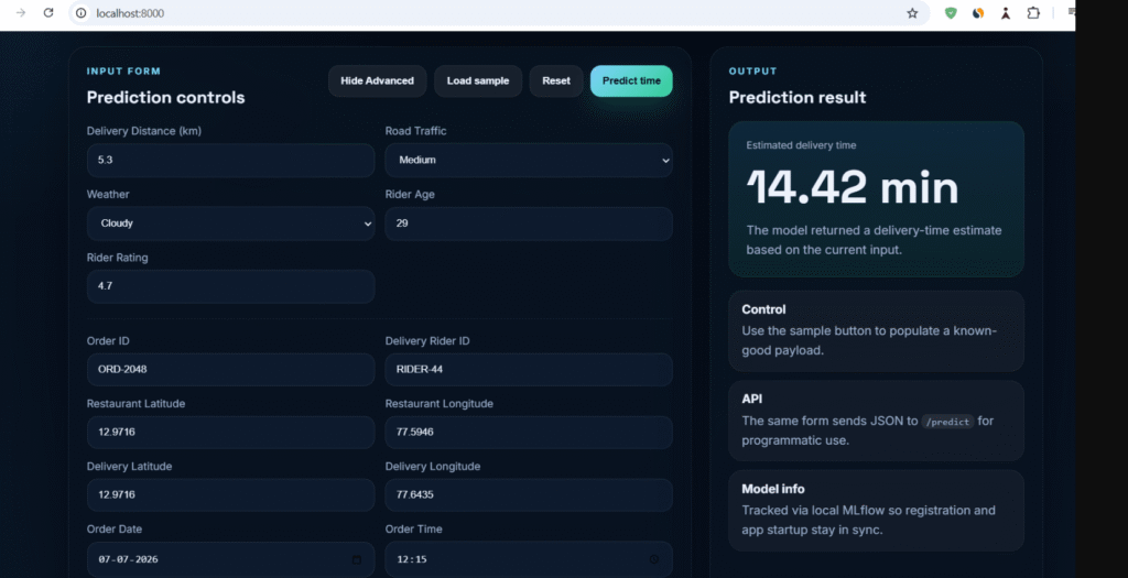
The project goes beyond simply training a machine learning model. It covers the complete workflow from raw data processing and feature engineering to model training, evaluation, experiment tracking, model management, API serving, containerization, and deployment.
The main objective is to build a practical, reproducible, and production-oriented machine learning system for predicting food delivery time.
1. What Problem Are We Solving? #
Food delivery time depends on many real-world factors.
For example:
- Traffic conditions
- Weather conditions
- Delivery distance
- Rider information
- Vehicle condition
- Restaurant location
- Delivery location
- Order time
- Pickup duration
- Number of deliveries
- Festival conditions
- City type
Because these factors can affect how long an order takes to reach the customer, predicting delivery time is not a simple rule-based problem.
Project Goal #
The goal of this project is:
Predict the food delivery time in minutes using information available about the delivery.
The target variable is a continuous numerical value representing delivery time.
Therefore, this problem is treated as a regression problem.
2. Why Is Delivery-Time Prediction Important? #
Estimated delivery time is an important part of the food-delivery experience.
When a customer places an order, they want to know approximately when the food will arrive.
An inaccurate prediction can lead to:
- Poor customer expectations
- Reduced customer satisfaction
- Inefficient delivery planning
- Difficulty identifying potentially delayed orders
A machine learning-based prediction system can help estimate delivery time more intelligently by learning patterns from historical delivery data.
Customer #
Accurate delivery-time estimates help customers understand when they can expect their food.
For example, instead of providing a generic delivery estimate, the system can consider the specific conditions of an order.
Rider Dispatch #
Delivery-time predictions can support better rider assignment and delivery planning.
The system can help identify deliveries that may require more time based on factors such as traffic, distance, and pickup duration.
Operations #
The business can use predictions to identify deliveries that may experience delays and take appropriate operational actions.
3. Machine Learning Solution #
Instead of manually defining rules for every possible delivery situation, the system learns patterns from historical delivery data.
The overall workflow can be understood as:
The project is designed as an end-to-end pipeline, rather than only a machine learning notebook.
This means the system considers the complete journey of the model:
Raw Data → Cleaning → Feature Engineering → Preprocessing → Training → Evaluation → Model Tracking → Model Registry → API → Deployment
This approach makes the project more suitable for real-world machine learning applications.
4. End-to-End System Architecture #
The project follows an MLOps-oriented architecture.
The workflow starts with raw delivery data and continues through multiple stages:
- Raw Data
- Data Versioning
- Data Cleaning
- Feature Engineering
- Data Preprocessing
- Model Training
- Model Evaluation
- Experiment Tracking
- Model Registry
- API Serving
- Containerization
- Deployment
Technologies Used #
The project combines several technologies:
- Python for machine learning and data processing
- Pandas and NumPy for data manipulation
- Scikit-learn for preprocessing and machine learning
- LightGBM for gradient boosting
- MLflow for experiment tracking and model management
- DVC for reproducible data pipelines
- FastAPI for model serving
- Docker for containerization
The important idea is that each technology solves a different part of the machine learning lifecycle.
5. Data Processing Pipeline #
The data processing pipeline prepares raw delivery data for machine learning.
The major stages are:
| Stage | Purpose | Output |
|---|---|---|
| Data Cleaning | Remove invalid and inconsistent data | Cleaned dataset |
| Data Preparation | Prepare data for machine learning | Training and testing data |
| Feature Engineering | Create useful features | Engineered dataset |
| Preprocessing | Transform numerical and categorical features | Processed features |
| Training | Train the regression model | Trained model |
| Evaluation | Measure model performance | Evaluation results |
| Model Registry | Store and manage the model | Registered model |
Using separate stages makes the workflow easier to reproduce and maintain.
6. Data Cleaning #
Before training the machine learning model, the raw Swiggy delivery dataset needs to be cleaned and transformed into a useful format.
The main data-preparation steps are:
- Standardize column names
- Handle missing values
- Clean invalid rider and rating values
- Clean latitude and longitude
- Create date-based features
- Create pickup-time features
- Create time-of-day features
- Clean categorical features
- Calculate delivery distance
- Combine everything into a reusable preprocessing pipeline
The goal is to convert raw delivery data into a clean and machine-learning-ready dataset.
6.1 Standardizing Column Names #
The original dataset contains column names such as:
Delivery_person_AgeDelivery_person_RatingsRestaurant_latitudeRestaurant_longitudeTime_taken(min)
Working with inconsistent column names can make the code harder to maintain. Therefore, the column names are converted into a consistent lowercase naming convention.
Code #
def change_column_names(data: pd.DataFrame) -> pd.DataFrame:
    """
    Standardize the dataset column names.

    The original dataset contains long and inconsistent
    column names. We rename them into shorter,
    consistent names that are easier to use.
    """

    # Mapping of original column names to new column names
    rename_dict = {
        'ID': 'id',
        'Delivery_person_ID': 'rider_id',
        'Delivery_person_Age': 'age',
        'Delivery_person_Ratings': 'ratings',
        'Restaurant_latitude': 'restaurant_latitude',
        'Restaurant_longitude': 'restaurant_longitude',
        'Delivery_latitude': 'delivery_latitude',
        'Delivery_longitude': 'delivery_longitude',
        'Order_Date': 'order_date',
        'Time_Orderd': 'order_time',
        'Time_Order_picked': 'order_picked_time',
        'Weatherconditions': 'weather',
        'Road_traffic_density': 'traffic',
        'Vehicle_condition': 'vehicle_condition',
        'Type_of_order': 'type_of_order',
        'Type_of_vehicle': 'type_of_vehicle',
        'multiple_deliveries': 'multiple_deliveries',
        'Festival': 'festival',
        'City': 'city_type',
        'Time_taken(min)': 'time_taken'
    }

    # Rename known columns.
    # If a column is not in rename_dict, convert it to lowercase.
    return data.rename(
        columns=lambda col: rename_dict.get(col, col.lower())
    )
Why do this? #
Consistent column names make later operations easier.
For example: Delivery_person_Age becomes: age
This makes the dataset easier to understand and reduces unnecessary typing throughout the project.
6.2 Handling Missing Values #
The dataset contains missing values represented as strings such as NaN.
These string values need to be converted into actual NumPy missing values so that Pandas and Scikit-learn can handle them correctly.
Code #
# Convert string representations of NaN into actual
# NumPy missing values.
df = df.replace(
    r'^\s*NaN\s*$',
    np.nan,
    regex=True
)
Why? #
There is an important difference between:
"NaN"→ a stringnp.nan→ an actual missing numerical value
Converting the string into np.nan allows standard missing-value operations to work correctly.
6.3 Cleaning Invalid Rider and Rating Values #
- The dataset contains rider age and rating information.
- Before using these features, they are converted into numerical values.
- Invalid records are then identified.
For this project:
- Rider age below 18 is considered anomalous.
- Ratings greater than 5 are considered invalid.
Code #
# Convert rider age into a numeric value.
# Invalid values are converted to NaN instead of causing an error.
df['age'] = pd.to_numeric(
    df['age'],
    errors='coerce'
)

# Convert rider ratings into numeric values.
# Invalid values are converted to NaN.
df['ratings'] = pd.to_numeric(
    df['ratings'],
    errors='coerce'
)

# Create a validation mask.
#
# Keep rows where:
# 1. Age is missing OR age is at least 18
# 2. Rating is missing OR rating is at most 5
valid_mask = (
    (df['age'].isna() | (df['age'] >= 18)) &
    (df['ratings'].isna() | (df['ratings'] <= 5.0))
)

# Keep only valid records.
df = df[valid_mask].copy()
Why use errors='coerce'? #
If a column contains an invalid value such as text where a number is expected, errors='coerce' converts that value into NaN instead of stopping the entire program with an error.
6.4 Cleaning Latitude and Longitude #
The dataset contains geographical coordinates for both:
- Restaurant
- Delivery location
These coordinates are later used to calculate delivery distance.
Some coordinate values may be invalid. Therefore, values below the selected threshold are replaced with missing values.
Code #
def clean_lat_long(
    data: pd.DataFrame,
    threshold: float = 1.0
) -> pd.DataFrame:

    # Columns containing geographical coordinates
    location_columns = [
        'restaurant_latitude',
        'restaurant_longitude',
        'delivery_latitude',
        'delivery_longitude'
    ]

    # Create a copy so that the original DataFrame
    # is not modified directly.
    df_out = data.copy()

    # Process every location column.
    for col in location_columns:

        # Make sure the column exists before processing it.
        if col in df_out.columns:

            # Replace values below the threshold with NaN.
            df_out[col] = np.where(
                df_out[col] < threshold,
                np.nan,
                df_out[col]
            )

    return df_out
Why clean geographical data? #
Incorrect latitude or longitude values can produce incorrect distance calculations.
Since distance is an important feature in this project, invalid coordinates should be handled before calculating distance.
6.5 Creating Date Features #
The original dataset contains an order date.
Instead of using the complete date directly, useful features are extracted from it.
The project creates:
- Order day
- Order month
- Day of week
- Weekend indicator
Code #
# Convert the order_date column into a datetime object.
#
# dayfirst=True is used because the dataset contains
# dates where the day appears before the month.
df['order_date'] = pd.to_datetime(
    df['order_date'],
    dayfirst=True,
    errors='coerce'
)

# Extract the day of the month.
df['order_day'] = df['order_date'].dt.day

# Extract the month.
df['order_month'] = df['order_date'].dt.month

# Extract the name of the day.
# Convert it to lowercase for consistency.
df['order_day_of_week'] = (
    df['order_date']
    .dt.day_name()
    .str.lower()
)

# Create a weekend indicator.
#
# Saturday and Sunday = 1
# Other days = 0
df['is_weekend'] = (
    df['order_date']
    .dt.day_name()
    .isin(['Saturday', 'Sunday'])
    .astype(int)
)
Why create these features? #
Delivery behavior can vary depending on the day.
For example:
- Weekdays may have different traffic patterns.
- Weekends may have different order volumes.
- Certain months may have different delivery behavior.
Instead of giving the model only the raw date, we extract information that may be more useful for prediction.
6.6 Creating Pickup-Time Features #
The project calculates how much time passes between:
Order Placed → Order Picked Up
This creates a new feature: pickup_time_minutes
Code #
# Convert order time into datetime format.
df['order_time_dt'] = pd.to_datetime(
    df['order_time'],
    format='mixed',
    errors='coerce'
)

# Convert order pickup time into datetime format.
df['order_picked_time_dt'] = pd.to_datetime(
    df['order_picked_time'],
    format='mixed',
    errors='coerce'
)

# Calculate the difference between pickup time
# and order time.
#
# total_seconds() converts the time difference
# into seconds, and dividing by 60 converts it
# into minutes.
df['pickup_time_minutes'] = (
    df['order_picked_time_dt']
    - df['order_time_dt']
).dt.total_seconds() / 60.0
Why is pickup time important? #
Total delivery time is not only affected by the distance between the restaurant and customer.
The restaurant may also take time to prepare the order.
Therefore: Longer pickup time → Potentially longer total delivery time
This makes pickup_time_minutes a useful engineered feature.
6.7 Creating Time-of-Day Features #
The order time is converted into an hour.
The hour is then grouped into meaningful categories:
- Morning
- Afternoon
- Evening
- Night
- After midnight
Code #
def time_of_day(hour_series: pd.Series) -> pd.Series:

    # Define the time ranges.
    conditions = [
        hour_series.between(6, 12, inclusive='left'),
        hour_series.between(12, 17, inclusive='left'),
        hour_series.between(17, 20, inclusive='left'),
        hour_series.between(20, 24, inclusive='left')
    ]

    # Assign a category to each time range.
    choices = [
        "morning",
        "afternoon",
        "evening",
        "night"
    ]

    # Select the appropriate category.
    # If none of the conditions match,
    # assign "after_midnight".
    return pd.Series(
        np.select(
            conditions,
            choices,
            default="after_midnight"
        ),
        index=hour_series.index
    )


# Extract the hour from the order datetime.
df['order_time_hour'] = (
    df['order_time_dt'].dt.hour
)

# Convert the hour into a time-of-day category.
df['order_time_of_day'] = time_of_day(
    df['order_time_hour']
)
Why create a time-of-day feature? #
Delivery conditions can change throughout the day.
For example: Morning → Afternoon → Evening → Night
may have different:
- Traffic
- Restaurant activity
- Order volume
- Rider availability
The categorical feature allows the model to learn these patterns.
6.8 Cleaning Categorical Features #
The dataset contains several categorical columns.
Examples include:
- Weather
- Traffic
- Vehicle type
These values are cleaned by:
- Removing unnecessary spaces
- Converting values to lowercase
- Removing unwanted prefixes
- Converting invalid string representations into missing values
Code #
# Clean the weather column.
df['weather'] = (
    df['weather']
    .astype(str)

    # Remove the unnecessary "conditions" prefix.
    .str.replace(
        r'^conditions\s+',
        '',
        regex=True
    )

    # Remove leading and trailing spaces.
    .str.strip()

    # Convert all values to lowercase.
    .str.lower()

    # Convert string representations of missing values
    # into actual NaN values.
    .replace(['nan', 'none', ''], np.nan)
)


# Clean the traffic column.
df['traffic'] = (
    df['traffic']
    .astype(str)
    .str.strip()
    .str.lower()
    .replace(['nan', 'none', ''], np.nan)
)


# Clean the vehicle-type column.
df['type_of_vehicle'] = (
    df['type_of_vehicle']
    .astype(str)
    .str.strip()
    .str.lower()
    .replace(['nan', 'none', ''], np.nan)
)
Why clean categorical data? #
Suppose the dataset contains:
SunnysunnySUNNY
These values represent the same category but could be treated as different values if they are not standardized.
Cleaning them ensures consistent categorical representation.
The time_taken column is cleaned by removing "(min)" and converting the values from string to integer so the machine learning model can use it as a numerical target. The order_time and order_picked_time columns are then removed because they are no longer needed after feature engineering.
# target column modifications
time_taken = lambda x: (
    x['time_taken']
    .str.replace("(min) ", "")
    .astype(int)
)
.drop(columns=["order_time", "order_picked_time"])
Food Delivery Time Analysis Using Exploratory Data Analysis #
Introduction #
Before training any machine learning model, you must understand your data deeply. EDA (Exploratory Data Analysis) is the process of:
- Understanding the shape, types, and quality of your data
- Discovering patterns and relationships between features
- Identifying anomalies and missing values
- Forming hypotheses that guide feature engineering and model selection
In this blog, we walk through the complete EDA of the Swiggy food delivery dataset — a real-world dataset containing information about delivery riders, orders, locations, and delivery times.
Our goal: Predict time_taken — the total delivery time in minutes.
Let’s explore every feature, one by one.
# import package
import numpy as np
import pandas as pd
import matplotlib.pyplot as plt
from matplotlib.gridspec import GridSpec
import seaborn as sns
import data_clean_utils
from scipy.stats import chi2_contingency, f_oneway, jarque_bera, probplot
import plotly.express as px
Why these libraries?
| Library | Purpose |
|---|---|
pandas / numpy | Data manipulation and numerical operations |
matplotlib / seaborn | Static visualizations (distributions, box plots, scatter plots) |
plotly.express | Interactive map visualizations |
scipy.stats | Statistical hypothesis tests (ANOVA, Chi-Square, Jarque-Bera) |
missingno | Visualizing missing data patterns |
data_clean_utils -Here Click For Code | Custom cleaning utility script (written separately) |
2. Load the Raw Data
# Load raw dataset
df = pd.read_csv('swiggy.csv')
df.sample(30)
3. Data Cleaning #
We perform data cleaning using a custom utility that handles:
- Fixing data type issues
- Extracting date/time features from raw datetime columns
- Handling 0-value coordinates (0° lat/lon is technically in the ocean — not India)
- Computing the Haversine distance between restaurant and delivery location
# Clean the data using the utility script
data_clean_utils.perform_data_cleaning(data=df)
# Load the cleaned output
df_final = pd.read_csv('swiggy_cleaned.csv')
4. Preliminary Analysis #
Shape and Structure #
df_final.isnull().sum()
# Count rows with at least one missing value
missing_rows = (
    df_final
    .isnull()
    .any(axis=1)
    .sum()
)

print(f'There are {missing_rows} rows with missing values in the data.')
print(f"It accounts for {(missing_rows/df_final.shape[0])*100:.2f}% of the data")
Key finding: The initial percentage of missing data was 9.2% but increased to 16.35% after cleaning — because we correctly converted invalid 0.0 latitude/longitude values (which geographically land in the Atlantic Ocean) to NaN.
# Check for duplicates
df_final.duplicated().sum()
# No duplicate rows in the dataset.
df_final.dtypes

# Separate numerical and categorical columns
num_cols = df_final.columns[[1, 2, 3, 4, 5, 6, 16, 22, 25]].tolist()
cat_cols  = [col for col in df_final.columns.tolist() if col not in num_cols]

print(f'There are {len(num_cols)} numerical columns and {len(cat_cols)} categorical columns.')
# Statistical Summary
# Numerical columns
df_final[num_cols].describe()
# Categorical columns
(
    df_final
    .assign(**{col: df_final[col].astype("object") for col in cat_cols})
    .describe(include="object")
    .T
)
5. Missing Value Analysis #
Understanding where and why data is missing is crucial. We use the missingno library for three complementary views.
Matrix Plot #
import missingno as msno

msno.matrix(df_final)
The matrix plot shows each row of the dataframe as a horizontal line. White gaps indicate missing values. This lets you see which columns tend to be missing together — a pattern called co-occurrence.
msno.heatmap(df_final)
The missingno heatmap shows how strongly the missingness of one column is correlated with another. A high correlation (close to 1) means whenever column A is missing, column B is also likely missing — suggesting a common cause (e.g., both come from the same source).
#Dendrogram
msno.dendrogram(df_final)
The dendrogram clusters columns by their missing-value correlation. Columns grouped close together have similar missingness patterns — helpful when deciding whether to impute together or separately.
Takeaway: Missing values in latitude/longitude columns co-occur heavily (they come from the same GPS source). Missing rider ratings and age appear independently.
6. Reusable Analysis Functions #
Rather than repeating plotting code 40+ times, we built four reusable analysis functions:
numerical_analysis — Understand a Continuous Variable
def numerical_analysis(dataframe, column_name, cat_col=None, bins="auto"):
    fig = plt.figure(figsize=(15, 10))
    grid = GridSpec(nrows=2, ncols=2, figure=fig)

    ax1 = fig.add_subplot(grid[0, 0])  # KDE Plot
    ax2 = fig.add_subplot(grid[0, 1])  # Box Plot
    ax3 = fig.add_subplot(grid[1, :])  # Full-width Histogram

    sns.kdeplot(data=dataframe, x=column_name, hue=cat_col, ax=ax1)
    sns.boxplot(data=dataframe, x=column_name, hue=cat_col, ax=ax2)
    sns.histplot(data=dataframe, x=column_name, bins=bins, hue=cat_col, kde=True, ax=ax3)

    plt.tight_layout()
    plt.show()
Why three plots? KDE reveals the smooth distribution shape; box plot highlights outliers and quartiles; histogram shows the raw frequency counts. Together, they give a complete picture.
# numerical_categorical_analysis — Num vs Category

def numerical_categorical_analysis(dataframe, cat_column_1, num_column):
    fig, (ax1, ax2) = plt.subplots(2, 2, figsize=(15, 7.5))

    sns.barplot(data=dataframe,   x=cat_column_1, y=num_column, ax=ax1[0])  # Mean per group
    sns.boxplot(data=dataframe,   x=cat_column_1, y=num_column, ax=ax1[1])  # Quartiles per group
    sns.violinplot(data=dataframe,x=cat_column_1, y=num_column, ax=ax2[0])  # Full distribution shape
    sns.stripplot(data=dataframe, x=cat_column_1, y=num_column, ax=ax2[1])  # Raw data points

    plt.tight_layout()
    plt.show()
#categorical_analysis — Understand a Category Variable

def categorical_analysis(dataframe, column_name):
    # Show counts and percentages
    display(
        pd.DataFrame({
            "Count": dataframe[column_name].value_counts(),
            "Percentage": (
                dataframe[column_name]
                .value_counts(normalize=True)
                .mul(100).round(2)
                .astype("str").add("%")
            )
        })
    )

    print("*" * 50)
    unique_categories = dataframe[column_name].unique().tolist()
    print(f"Unique categories in {column_name}: {unique_categories}")
    print(f"Number of categories: {dataframe[column_name].nunique()}")

    sns.countplot(data=dataframe, x=column_name)
    plt.xticks(rotation=45)
    plt.show()
multivariate_analysis — Two Categories vs One Numeric
def multivariate_analysis(dataframe, num_column, cat_column_1, cat_column_2):
    fig, (ax1, ax2) = plt.subplots(2, 2, figsize=(15, 7.5))

    sns.barplot(data=dataframe,    x=cat_column_1, y=num_column, hue=cat_column_2, ax=ax1[0])
    sns.boxplot(data=dataframe,    x=cat_column_1, y=num_column, hue=cat_column_2, gap=0.1, ax=ax1[1])
    sns.violinplot(data=dataframe, x=cat_column_1, y=num_column, hue=cat_column_2, gap=0.1, ax=ax2[0])
    sns.stripplot(data=dataframe,  x=cat_column_1, y=num_column, hue=cat_column_2, dodge=True, ax=ax2[1])

    plt.tight_layout()
    plt.show()
Hypothesis Testing Functions
def anova_test(dataframe, num_col, cat_col, alpha=0.05):
    """One-Way ANOVA: Does the mean of num_col differ across cat_col groups?"""
    groups = [
        group[num_col].dropna().values
        for _, group in dataframe.groupby(cat_col)
    ]
    stat, p_value = f_oneway(*groups)
    print(f"F-statistic: {stat:.4f}, p-value: {p_value:.6f}")
    if p_value < alpha:
        print(f"✅ Reject H₀ — '{cat_col}' significantly affects '{num_col}'")
    else:
        print(f"❌ Fail to reject H₀ — '{cat_col}' does NOT significantly affect '{num_col}'")


def chi_2_test(dataframe, col1, col2, alpha=0.05):
    """Chi-Square Test: Are two categorical variables independent?"""
    contingency = pd.crosstab(dataframe[col1], dataframe[col2])
    chi2, p, dof, expected = chi2_contingency(contingency)
    print(f"Chi2: {chi2:.4f}, p-value: {p:.6f}, df: {dof}")
    if p < alpha:
        print(f"✅ Reject H₀ — '{col1}' and '{col2}' are NOT independent (related)")
    else:
        print(f"❌ Fail to reject H₀ — '{col1}' and '{col2}' are independent")


def test_for_normality(dataframe, column, alpha=0.05):
    """Jarque-Bera test for normality."""
    stat, p = jarque_bera(dataframe[column].dropna())
    print(f"JB-statistic: {stat:.4f}, p-value: {p:.6f}")
    if p < alpha:
        print(f"❌ '{column}' is NOT normally distributed")
    else:
        print(f"✅ '{column}' appears normally distributed")
7. Column-Wise EDA #
7.1 Target Column: time_taken #
The most important column in any ML project is the target. Let’s understand it deeply.
# Numerical analysis of delivery time
numerical_analysis(df_final, 'time_taken', bins=10)
Observations:
time_takenis not fully continuous — it behaves like a discretized variable (riders likely round to the nearest minute)- It shows bimodality with two peaks — one around 17–18 minutes and another around 26–27 minutes, suggesting two distinct delivery scenarios (short local vs. longer cross-city)
- There are extreme values near 50 minutes — these are not true outliers, just rare but valid long deliveries
# Q-Q Plot to visually assess normality
from scipy.stats import probplot

probplot(df_final['time_taken'], plot=plt)
plt.show()

# Statistical test for normality
test_for_normality(df_final, 'time_taken')
Finding: The Q-Q plot shows significant deviation from the diagonal, and the Jarque-Bera test confirms time_taken is not normally distributed. This is why we’ll apply a PowerTransformer later.
Are the Extreme Values Really Outliers? #
# Compute IQR bounds
target_25, target_75 = np.percentile(df_final['time_taken'], [25, 75])
iqr = target_75 - target_25
upper_bound = target_75 + (1.5 * iqr)

# What traffic conditions do extreme-time orders have?
df_final.loc[df_final['time_taken'] > upper_bound, "traffic"].value_counts()
# What weather conditions?
df_final.loc[df_final['time_taken'] > upper_bound, "weather"].value_counts()
# Are extreme-time orders covering longer distances?
avg_distance         = df_final["distance"].mean()
avg_distance_extreme = df_final.loc[df_final['time_taken'] > upper_bound, "distance"].mean()

print(f"Overall avg distance:       {avg_distance:.2f} km")
print(f"Extreme-time avg distance:  {avg_distance_extreme:.2f} km")
Conclusion: The high-time deliveries tend to be during heavy traffic, bad weather, and longer distances. They are genuine real-world cases — not data entry errors. We keep them.
# Fixing the Skewness with PowerTransformer
from sklearn.preprocessing import PowerTransformer

pt = PowerTransformer(method='yeo-johnson')
df_final['time_taken_pt'] = pt.fit_transform(df_final[['time_taken']])

# Visualize after transformation
numerical_analysis(df_final, "time_taken_pt", bins=10)

# Q-Q plot after transformation
probplot(df_final['time_taken_pt'], plot=plt)
plt.show()
Result: After Yeo-Johnson transformation, the distribution is much closer to Gaussian — the Q-Q plot aligns well with the diagonal. This will be used as the training target in Part 2.
df_final[["rider_id", "age", "ratings"]].groupby('rider_id').head(5).sort_values('rider_id')

# Check if a rider appears with different ages/ratings
df_final[["rider_id", "age", "ratings"]].dropna().duplicated(keep=False).sum()
Finding: rider_id is a unique identifier. It provides no predictive signal for delivery time and will be dropped before modelling.
# Rider Age
# Statistical summary
df_final['age'].describe()

# Distribution analysis
numerical_analysis(df_final, 'age', bins=20)

# Relationship between age and delivery time
sns.scatterplot(data=df_final, x='age', y='time_taken')
plt.show()
Finding: Age shows no meaningful relationship with delivery time. The scatter plot shows a uniform cloud with no trend. However, age may interact with vehicle condition — younger riders may maintain their vehicles better.
# Does vehicle condition vary with age?
sns.scatterplot(data=df_final, x='age', y='time_taken', hue="vehicle_condition")
plt.legend(bbox_to_anchor=(1.02, 1), loc=2)
plt.show()

# Vehicle type preferences by age
sns.stripplot(df_final, x='type_of_vehicle', y='age')
plt.show()
Finding: Different age groups prefer different vehicle types, but age alone doesn’t drive delivery time. We include it as a feature to let the model decide its importance.
# Rider Rating
df_final['ratings'].describe()

# Distribution
numerical_analysis(df_final, 'ratings', bins=5)

# Does ratings affect delivery time?
sns.scatterplot(data=df_final, x='ratings', y='time_taken')
plt.show()
Observation: Riders with higher ratings tend to receive more orders, suggesting ratings act as a proxy for rider experience and reliability.
# Does vehicle condition affect ratings?
numerical_categorical_analysis(df_final, 'vehicle_condition', 'ratings')
Finding: Riders with worse vehicle condition (vehicle_condition = 3) receive lower ratings on average. Interestingly, this category has NaN ratings — suggesting customers don’t even bother rating when the vehicle is in terrible condition.
# Check vehicle condition = 3 ratings distribution
(
    df_final[["ratings", "vehicle_condition"]]
    .loc[df_final["vehicle_condition"] == 3, "ratings"]
    .value_counts(dropna=False)
)

# Does vehicle type affect ratings?
numerical_categorical_analysis(df_final, 'type_of_vehicle', 'ratings')

# Does festival affect ratings?
numerical_categorical_analysis(df_final, 'festival', 'ratings')
Insight: The delivery points cluster around major Indian cities — Mumbai, Delhi, Bangalore, Hyderabad, Chennai. This confirms the dataset covers metropolitan delivery operations.
Note on coordinates: Raw latitude/longitude won’t be used directly as model features. Instead, we computed the Haversine distance between the restaurant and delivery coordinates during data cleaning — a single, meaningful numerical feature that captures the geographic relationship.
7.5 📍 Location-Based Features
# Location data subset
location_subset = df_final.loc[:, df_final.columns[3:7].tolist() + ["city_name"]]
location_subset.dropna(inplace=True)

# Interactive Delivery Map
delivery_df = pd.DataFrame({
    'latitude':  location_subset['delivery_latitude'],
    'longitude': location_subset['delivery_longitude'],
    'city_name': location_subset['city_name']
})

fig = px.scatter_mapbox(
    delivery_df,
    lat='latitude', lon='longitude',
    title="Delivery Points Across India",
    hover_name="city_name"
)

fig.update_layout(
    mapbox_style="carto-positron",
    mapbox_center={"lat": 20.5937, "lon": 78.9629},  # Center of India
    mapbox_zoom=3,
)
fig.show()
7.6 Order Date, Day & Weekend
# Time-related columns
order_date_subset = df_final.loc[:, [
    "order_date", "order_day", "order_month",
    "order_day_of_week", "is_weekend", "festival"
]]
Does Day of Week Matter?
numerical_categorical_analysis(df_final, "order_day_of_week", "time_taken")
Finding: Delivery times are relatively consistent across days of the week with no dramatic differences. Day-of-week alone is not a strong predictor.
# Do Weekends Take Longer?
numerical_categorical_analysis(df_final, "is_weekend", "time_taken")

# Does weekend affect traffic?
chi_2_test(df_final, "is_weekend", "traffic")
Finding: Weekends show a slight increase in delivery time. The Chi-Square test confirms weekends significantly affect traffic patterns — more leisure travel leads to heavier traffic on weekends.
numerical_categorical_analysis(df_final, "festival", "time_taken")
Observations:
- Average delivery time is higher during festivals
- The range of delivery time is narrower during festivals — less variation because nearly all deliveries are slowed down uniformly
- This makes festivals an important categorical signal for the model
# Do festivals affect traffic?
chi_2_test(df_final, "festival", "traffic")
The p-value is extremely small → festivals significantly affect traffic.
# Pivot table: average delivery time by traffic × festival
df_final.pivot_table(
    index="traffic",
    columns="festival",
    values="time_taken",
    aggfunc="mean"
)
| traffic | No Festival | Festival |
|---|---|---|
| low | 20.1 | 22.3 |
| medium | 23.4 | 25.8 |
| high | 26.7 | 29.1 |
| jam | 30.2 | 33.4 |
Pattern: At every traffic level, festival deliveries take ~2–3 minutes longer on average.
# Combined effect: weekend + festival on delivery time
multivariate_analysis(df_final, "time_taken", "is_weekend", "festival")
7.7 Order Time of Day #
# Time-related features
time_subset = df_final.loc[:, ["order_time_hour", "order_time_of_day", "pickup_time_minutes"]]

# Does time of day affect delivery time?
numerical_categorical_analysis(df_final, "order_time_of_day", "time_taken")

# ANOVA test: Is the difference statistically significant?
anova_test(df_final, "time_taken", "order_time_of_day")

# Which hours have the most orders?
df_final["order_time_hour"].value_counts().head(5)

# Distribution of orders by hour
categorical_analysis(df_final, "order_time_hour")

# Distribution by time of day bucket
categorical_analysis(df_final, "order_time_of_day")
Finding: ANOVA confirms time of day has a statistically significant effect on delivery time. Dinner orders (evening) tend to take longer — likely due to peak traffic and higher order volumes. The order_time_of_day (morning/afternoon/evening/night) is used as an engineered feature rather than the raw hour.
7.8 Pickup Time #
pickup_time_minutes = time the rider waits at the restaurant before picking up the order.
# Relationship between pickup time and delivery time
sns.scatterplot(df_final, x="pickup_time_minutes", y="time_taken")
plt.show()

# Does pickup time (as category) affect delivery time?
numerical_categorical_analysis(df_final, "pickup_time_minutes", "time_taken")
# ANOVA test
anova_test(df_final, "time_taken", "pickup_time_minutes")
Key Insight: Pickup time has a direct and strong relationship with total delivery time — every minute waiting at the restaurant adds a minute to the total. ANOVA confirms this is highly significant. pickup_time_minutes is one of our most important features.
7.9 Traffic Conditions #
# Distribution of traffic conditions
categorical_analysis(df_final, "traffic")

# Does traffic level depend on city type?
chi_2_test(df_final, "traffic", "city_type")

# Does traffic level depend on specific city?
chi_2_test(df_final, "traffic", "city_name")
Finding: Traffic distribution is significantly different across city types and individual cities — metropolitan cities have higher jam frequencies than semi-urban areas.
# Does traffic affect delivery time?
numerical_categorical_analysis(df_final, "traffic", "time_taken")

# ANOVA test
anova_test(df_final, "time_taken", "traffic")
Finding: Traffic is the second most impactful feature after distance. ANOVA strongly confirms that delivery time increases monotonically: low → medium → high → jam.
# Are some vehicles better in traffic?
multivariate_analysis(df_final, "time_taken", "traffic", "type_of_vehicle")

# Does vehicle condition interact with traffic?
multivariate_analysis(df_final, "time_taken", "traffic", "vehicle_condition")
⚠️ Don’t misinterpret! If the chart shows “better vehicle condition = longer delivery time,” this is a confounding effect — not causation. Better-condition vehicles are preferred for festival deliveries (which inherently take longer). See below:
# Confirm: good vehicles used more during festivals
multivariate_analysis(df_final, "time_taken", "festival", "vehicle_condition")
7.10 Multiple Deliveries #
# Does batching multiple orders affect delivery time?
numerical_categorical_analysis(df_final, "multiple_deliveries", "time_taken")

# ANOVA test
anova_test(df_final, "time_taken", "multiple_deliveries")

# Are multiple-delivery orders covering more distance?
numerical_categorical_analysis(df_final, "multiple_deliveries", "distance")
Finding: Riders carrying multiple orders take significantly longer. ANOVA confirms this is statistically significant. Interestingly, multiple-delivery orders also tend to cover larger total distances — the rider must visit multiple drop points.
7.11 Weather Conditions #
# Weather distribution
categorical_analysis(df_final, "weather")

# Does weather affect delivery time?
numerical_categorical_analysis(df_final, "weather", "time_taken")

# ANOVA test
anova_test(df_final, "time_taken", "weather")

# Does weather affect traffic?
chi_2_test(df_final, "weather", "traffic")
Findings:
- ANOVA confirms weather significantly affects delivery time
- Chi-Square confirms weather and traffic are not independent — bad weather causes heavier traffic
- Rain/fog conditions see the longest deliveries
# Combined effect: weather × traffic on delivery time
multivariate_analysis(df_final, "time_taken", "weather", "traffic")

# Pivot table
df_final.pivot_table(
    index="weather",
    columns="traffic",
    values="time_taken",
    aggfunc="mean"
)
Key Insight: The combination of bad weather + heavy traffic is the worst case — delivery times in Stormy + Jam conditions are ~35% higher than Sunny + Low traffic. Traffic acts as the strongest discriminatory feature in combination with other variables.
7.12 Vehicle Condition & Type #
# Vehicle condition distribution
categorical_analysis(df_final, "vehicle_condition")

# Does condition affect delivery time?
numerical_categorical_analysis(df_final, "vehicle_condition", "time_taken")

# ANOVA test
anova_test(df_final, "time_taken", "vehicle_condition")

# Vehicle type distribution
categorical_analysis(df_final, "type_of_vehicle")

# Does type of vehicle affect delivery time?
numerical_categorical_analysis(df_final, "type_of_vehicle", "time_taken")

# Interaction: vehicle condition × vehicle type on delivery time
multivariate_analysis(df_final, "time_taken", "vehicle_condition", "type_of_vehicle")

# Are vehicle type and condition related?
chi_2_test(df_final, "type_of_vehicle", "vehicle_condition")
Findings:
- Vehicle condition affects delivery time — poorly maintained vehicles are slower
- Different vehicle types (scooter, motorcycle, bicycle, etc.) have different average speeds
- Chi-Square confirms vehicle type and condition are related — certain vehicle types are more likely to be in poor condition
7.13 Type of Order #
# Order type distribution
categorical_analysis(df_final, "type_of_order")

# Does order type affect delivery time?
numerical_categorical_analysis(df_final, "type_of_order", "time_taken")

# ANOVA test
anova_test(df_final, "time_taken", "type_of_order")

# Cross-tab: order type vs weekend
pd.crosstab(df_final["type_of_order"], df_final["is_weekend"])
# Does order type affect pickup time?
chi_2_test(df_final, "pickup_time_minutes", "type_of_order")

# Does order type affect ratings?
numerical_categorical_analysis(df_final, "type_of_order", "ratings")

# Weekend vs order type
chi_2_test(df_final, "is_weekend", "type_of_order")

# Festival vs order type
chi_2_test(df_final, "festival", "type_of_order")
Findings:
- Order type (Snacks, Meal, Drinks, Buffet) has a significant effect on delivery time
- Restaurant meal orders take the longest (higher preparation complexity)
- Certain order types are more popular on weekends and festivals
7.14 City Analysis #
# City name distribution
categorical_analysis(df_final, "city_name")

# Does city affect delivery time?
numerical_categorical_analysis(df_final, "city_name", "time_taken")

# City type distribution (metropolitan, urban, semi-urban)
categorical_analysis(df_final, "city_type")

# Does city type affect delivery time?
numerical_categorical_analysis(df_final, "city_type", "time_taken")

# ANOVA test
anova_test(df_final, "time_taken", "city_type")

# Does city type affect rider ratings?
numerical_categorical_analysis(df_final, "city_type", "ratings")

# Combined: city type × vehicle type on delivery time
multivariate_analysis(df_final, "time_taken", "city_type", "type_of_vehicle")
Findings:
- Metropolitan cities have slightly longer delivery times — denser traffic and longer distances to navigate
- City type significantly affects rider ratings — urban riders tend to have higher ratings (potentially due to better infrastructure and shorter delivery windows)
- Different vehicle types perform differently across city types (bicycles are slower in semi-urban spread-out areas)
7.15 Distance #
The Haversine distance between the restaurant and delivery location — computed during cleaning.
# Numerical analysis of distance
numerical_analysis(df_final, "distance", bins=10)

# Scatterplot: distance vs delivery time
sns.scatterplot(df_final, x="distance", y="time_taken")
plt.show()

# Correlation
df_final[["distance", "time_taken"]].corr()

# Does vehicle type affect the distances covered?
numerical_categorical_analysis(df_final, "type_of_vehicle", "distance")

# Do riders cover more distance during festivals?
numerical_categorical_analysis(df_final, "distance", "festival")

# Distance distribution by vehicle type
numerical_categorical_analysis(df_final, "distance", "type_of_vehicle")
Findings:
- Distance shows a positive correlation with delivery time — the strongest linear relationship of any single feature
- The scatter plot shows significant variance at each distance value, confirming that distance alone doesn’t explain everything (traffic, weather, pickup time all add noise)
- Festival deliveries tend to cover slightly greater distances — riders may accept orders from farther restaurants when order volumes are high
- Motorcycles and electric scooters cover the widest range of distances; bicycles are used predominantly for short distances
8. EDA Summary & Key Insights #
After exploring all features, here’s what we learned:
Top Predictors of Delivery Time #
| Feature | Impact | Nature |
|---|---|---|
distance | High | Strongest linear predictor |
traffic | High | Monotonic ordinal effect (low → jam) |
pickup_time_minutes | High | Every minute at restaurant = +1 to total |
festival | Medium | Adds ~2–3 min across all traffic levels |
weather | Medium | Bad weather compounds with traffic |
multiple_deliveries | Medium | Batching significantly increases time |
order_time_of_day | Medium | Evening orders take longest |
city_type | Medium | Metro cities → longer deliveries |
vehicle_condition | Low | Confounded with festival ordering patterns |
type_of_vehicle | Low | Moderate effect, varies by city type |
ratings | Low | Higher-rated = faster (indirect) |
age | None | No meaningful direct effect |
rider_id | None | Identifier, drop before modelling |
Important Feature Interactions #
- Traffic × Weather → Worst combination for delivery time
- Festival × Traffic → Festival amplifies traffic effect
- Multiple deliveries × Distance → Batched orders cover more ground
- Vehicle condition × Festival → Better vehicles used during festivals (confounding)
- Weekend × Traffic → Weekends increase traffic, which increases time
Preprocessing Decisions Made #
| Decision | Reason |
|---|---|
Convert time_taken with PowerTransformer | Right-skewed, non-normal distribution |
| Keep extreme delivery values | Real-world cases, not errors |
Drop raw lat/lon, use distance | Engineered feature is more meaningful |
Drop rider_id | Identifier, no predictive value |
Encode traffic as ordinal | Natural ordering: low < medium < high < jam |
Encode distance_type as ordinal | Natural ordering: short < medium < long < very_long |
| One-Hot Encode other categoricals | No natural ordering |
| Scale numerical features | Ensures distance doesn’t dominate other features |
Model Selection, Hyperparameter Tuning & The LightGBM Champion #
Introduction #
In Part 1 of this series, we cleaned the raw Swiggy dataset, handled missing values, and extracted rich features like distance, pickup_time_minutes, traffic, order_time_of_day, and more. We ended with a tidy swiggy_cleaned.csv ready for modelling.
In this part, we tackle the most exciting phase of any ML project:
- Setting up the preprocessing pipeline
- Model Selection — Comparing 6 candidate algorithms using Optuna
- Hyperparameter Tuning — Deep-dive tuning of the top contenders (Random Forest & LightGBM)
- Ensemble via Stacking — Combining the best two models
- The Winner: LightGBM — Final evaluation and what makes it shine
1. Loading the Cleaned Data #
We start by loading the cleaned dataset produced in Part 1:
import pandas as pd
import numpy as np
import mlflow
from sklearn.model_selection import train_test_split
from sklearn.preprocessing import PowerTransformer, MinMaxScaler, OneHotEncoder, OrdinalEncoder
from sklearn.compose import ColumnTransformer
from sklearn.pipeline import Pipeline

# load the cleaned data
df = pd.read_csv('swiggy_cleaned.csv')
df.shape  # (45,584 rows × 26 columns, approximately)
Drop Columns Not Needed for Modelling #
Several columns were useful for EDA but won’t help the model: raw coordinates, IDs, and time-parts that are already captured by engineered features:
columns_to_drop = [
    'rider_id',
    'restaurant_latitude', 'restaurant_longitude',
    'delivery_latitude', 'delivery_longitude',
    'order_date',
    'order_time_hour', 'order_day',
    'city_name', 'order_day_of_week', 'order_month'
]

df.drop(columns=columns_to_drop, inplace=True)
Why drop raw coordinates? We already engineered a distance column (Haversine distance between restaurant and delivery point). The raw lat/lon would only add noise and dimensionality without providing additional information.
2. Data Split & Target Transformation #
Train-Test Split #
We separate features (X) from the target (y = time_taken) and perform an 80/20 split:
# Drop rows with missing values (Experiment 1 approach)
temp_df = df.copy().dropna()

X = temp_df.drop(columns='time_taken')
y = temp_df['time_taken']

X_train, X_test, y_train, y_test = train_test_split(
    X, y, test_size=0.2, random_state=42
)

print("Train size:", X_train.shape)   # e.g. (36,000+, 14)
print("Test size:",  X_test.shape)    # e.g. (9,000+, 14)
Why Transform the Target? #
time_taken (delivery time in minutes) is right-skewed. Many ML algorithms (and especially loss functions) assume or perform better with normally-distributed targets.
We apply PowerTransformer (Yeo-Johnson), which makes the distribution closer to Gaussian:
from sklearn.preprocessing import PowerTransformer

pt = PowerTransformer()

# Fit ONLY on training data to avoid data leakage
y_train_pt = pt.fit_transform(y_train.values.reshape(-1, 1))
y_test_pt  = pt.transform(y_test.values.reshape(-1, 1))
⚠️ Data Leakage Warning: The PowerTransformer is fit only on y_train and then applied to y_test. Fitting on the full dataset before splitting would leak test information into training — a classic mistake.
3. Preprocessing Pipeline #
Feature Categories #
Our features fall into three types, each requiring different treatment:
| Type | Features | Transformation |
|---|---|---|
| Numerical | age, ratings, pickup_time_minutes, distance | MinMax Scaling |
| Nominal Categorical | weather, type_of_order, type_of_vehicle, festival, city_type, is_weekend, order_time_of_day | One-Hot Encoding |
| Ordinal Categorical | traffic, distance_type | Ordinal Encoding (with custom order) |
Ordinal Feature Orders #
Traffic and distance have natural orderings that we encode explicitly:
traffic_order       = ["low", "medium", "high", "jam"]
distance_type_order = ["short", "medium", "long", "very_long"]
Building the Preprocessor
num_cols = ["age", "ratings", "pickup_time_minutes", "distance"]

nominal_cat_cols = [
    'weather', 'type_of_order', 'type_of_vehicle',
    "festival", "city_type", "is_weekend", "order_time_of_day"
]

ordinal_cat_cols = ["traffic", "distance_type"]

preprocessor = ColumnTransformer(transformers=[
    ("scale",
     MinMaxScaler(),
     num_cols),

    ("nominal_encode",
     OneHotEncoder(drop="first", handle_unknown="ignore", sparse_output=False),
     nominal_cat_cols),

    ("ordinal_encode",
     OrdinalEncoder(
         categories=[traffic_order, distance_type_order],
         encoded_missing_value=-999,
         handle_unknown="use_encoded_value",
         unknown_value=-1
     ),
     ordinal_cat_cols)

], remainder="passthrough", n_jobs=-1,
   force_int_remainder_cols=False,
   verbose_feature_names_out=False)
Key design decisions:
drop="first"in OneHotEncoder avoids the dummy variable trap (multicollinearity)handle_unknown="ignore"makes the pipeline robust to unseen categories at inferenceencoded_missing_value=-999ensures NaN ordinal values get a sentinel — not confused with a valid category
Pipeline Assembly
processing_pipeline = Pipeline(steps=[
    ("preprocess", preprocessor)
])

# Fit on train, transform both
X_train_trans = processing_pipeline.fit_transform(X_train)
X_test_trans  = processing_pipeline.transform(X_test)
Model Selection with Optuna #
Rather than manually trying each algorithm one by one, we run a multi-model Optuna study — an automated hyperparameter search that also selects the type of model to use.
Why Optuna? #
Optuna uses Tree-structured Parzen Estimator (TPE) sampling — a Bayesian optimization technique that learns which configurations are promising and focuses the search there, unlike grid or random search that sample blindly.
from sklearn.ensemble import RandomForestRegressor, GradientBoostingRegressor
from sklearn.neighbors import KNeighborsRegressor
from sklearn.svm import SVR
from xgboost import XGBRegressor
from lightgbm import LGBMRegressor
import optuna

from sklearn.metrics import mean_absolute_error
from sklearn.model_selection import cross_val_score
from sklearn.compose import TransformedTargetRegressor
The Objective Function #
The objective function is the heart of Optuna. It:
- Picks a model type (trial parameter)
- Picks model-specific hyperparameters
- Trains and cross-validates
- Returns the metric to minimize (MAE)
def objective(trial):
    with mlflow.start_run(nested=True):

        model_name = trial.suggest_categorical(
            "model", ["SVM", "RF", "KNN", "GB", "XGB", "LGBM"]
        )

        # ── SVM ──────────────────────────────────────────────────────
        if model_name == "SVM":
            kernel_svm = trial.suggest_categorical(
                "kernel_svm", ["linear", "poly", "rbf"]
            )
            if kernel_svm == "linear":
                c_linear = trial.suggest_float("c_linear", 0, 10)
                model = SVR(C=c_linear, kernel="linear")

            elif kernel_svm == "poly":
                c_poly   = trial.suggest_float("c_poly", 0, 10)
                deg_poly = trial.suggest_int("degree_poly", 1, 5)
                model    = SVR(C=c_poly, degree=deg_poly, kernel="poly")

            else:  # rbf
                c_rbf    = trial.suggest_float("c_rbf", 0, 100)
                gamma    = trial.suggest_float("gamma_rbf", 0, 10)
                model    = SVR(C=c_rbf, gamma=gamma, kernel="rbf")

        # ── Random Forest ─────────────────────────────────────────────
        elif model_name == "RF":
            n_estimators_rf = trial.suggest_int("n_estimators_rf", 10, 200)
            max_depth_rf    = trial.suggest_int("max_depth_rf", 2, 20)
            model = RandomForestRegressor(
                n_estimators=n_estimators_rf,
                max_depth=max_depth_rf,
                random_state=42, n_jobs=-1
            )

        # ── Gradient Boosting ──────────────────────────────────────────
        elif model_name == "GB":
            n_estimators_gb  = trial.suggest_int("n_estimators_gb", 10, 200)
            learning_rate_gb = trial.suggest_float("learning_rate_gb", 0, 1)
            max_depth_gb     = trial.suggest_int("max_depth_gb", 2, 20)
            model = GradientBoostingRegressor(
                n_estimators=n_estimators_gb,
                learning_rate=learning_rate_gb,
                max_depth=max_depth_gb,
                random_state=42
            )

        # ── KNN ────────────────────────────────────────────────────────
        elif model_name == "KNN":
            n_neighbors_knn = trial.suggest_int("n_neighbors_knn", 1, 30)
            weights_knn     = trial.suggest_categorical(
                "weights_knn", ["uniform", "distance"]
            )
            model = KNeighborsRegressor(
                n_neighbors=n_neighbors_knn,
                weights=weights_knn, n_jobs=-1
            )

        # ── XGBoost ────────────────────────────────────────────────────
        elif model_name == "XGB":
            n_estimators_xgb  = trial.suggest_int("n_estimators_xgb", 10, 200)
            learning_rate_xgb = trial.suggest_float("learning_rate_xgb", 0, 1)
            max_depth_xgb     = trial.suggest_int("max_depth_xgb", 2, 20)
            model = XGBRegressor(
                n_estimators=n_estimators_xgb,
                learning_rate=learning_rate_xgb,
                max_depth=max_depth_xgb,
                random_state=42, n_jobs=-1, verbosity=0
            )

        # ── LightGBM ───────────────────────────────────────────────────
        else:  # LGBM
            n_estimators_lgbm  = trial.suggest_int("n_estimators_lgbm", 10, 200)
            learning_rate_lgbm = trial.suggest_float("learning_rate_lgbm", 0, 1)
            max_depth_lgbm     = trial.suggest_int("max_depth_lgbm", 2, 20)
            model = LGBMRegressor(
                n_estimators=n_estimators_lgbm,
                learning_rate=learning_rate_lgbm,
                max_depth=max_depth_lgbm,
                random_state=42, n_jobs=-1
            )

        # ── Wrap with target transformer ──────────────────────────────
        wrapped = TransformedTargetRegressor(regressor=model, transformer=pt)

        # ── 5-fold Cross Validation ───────────────────────────────────
        cv_scores = cross_val_score(
            wrapped, X_train_trans, y_train,
            cv=5, scoring="neg_mean_absolute_error", n_jobs=-1
        )
        mean_mae = -cv_scores.mean()

        mlflow.log_metric("cross_val_mae", mean_mae)
        return mean_mae
Running the Study
study = optuna.create_study(direction="minimize", study_name="model_selection")

with mlflow.start_run(run_name="Best Model") as parent:
    study.optimize(objective, n_trials=30, n_jobs=-1)
    mlflow.log_params(study.best_params)
    mlflow.log_metric("best_score", study.best_value)
Model Selection Results #
After 30 trials, we inspect which models performed best:
# Average MAE for each model type
study.trials_dataframe().groupby("params_model")['value'].mean().sort_values()
| Model | Average CV MAE (minutes) |
|---|---|
| LGBM | 4.71 |
| XGBoost | 4.89 |
| Random Forest | 5.02 |
| Gradient Boosting | 5.31 |
| KNN | 6.44 |
| SVM | 7.12 |
LightGBM and Random Forest clearly lead the pack. Both are tree-based ensemble methods that handle tabular data extremely well. We select these two for deep hyperparameter tuning.
# Visualize optimization history
optuna.visualization.plot_optimization_history(study)

# See model selection landscape
optuna.visualization.plot_parallel_coordinate(study, params=["model"])
5. Hyperparameter Tuning — Random Forest 🌲 #
Now we deep-dive into the Random Forest hyperparameter space with 20 Optuna trials, each scored by 5-fold cross-validation MAE.
Hyperparameter Search Space #
| Parameter | Range | Meaning |
|---|---|---|
n_estimators | 10 – 500 | Number of trees in the forest |
max_depth | 1 – 30 | Maximum depth of each tree |
max_features | None / sqrt / log2 | Features considered per split |
min_samples_split | 2 – 10 | Min samples to split an internal node |
min_samples_leaf | 1 – 10 | Min samples required at a leaf node |
max_samples | 0.5 – 1.0 | Fraction of training samples for each tree |
from sklearn.ensemble import RandomForestRegressor
import optuna

def objective(trial):
    with mlflow.start_run(nested=True):
        params = {
            "n_estimators":    trial.suggest_int("n_estimators", 10, 500),
            "max_depth":       trial.suggest_int("max_depth", 1, 30),
            "max_features":    trial.suggest_categorical("max_features",
                                                          [None, "sqrt", "log2"]),
            "min_samples_split": trial.suggest_int("min_samples_split", 2, 10),
            "min_samples_leaf":  trial.suggest_int("min_samples_leaf", 1, 10),
            "max_samples":     trial.suggest_float("max_samples", 0.5, 1.0),
            "random_state": 42,
            "n_jobs": -1,
        }

        mlflow.log_params(params)

        rf    = RandomForestRegressor(**params)
        model = TransformedTargetRegressor(regressor=rf, transformer=pt)
        model.fit(X_train_trans, y_train)

        # 5-fold CV
        cv_score  = cross_val_score(model, X_train_trans, y_train,
                                    cv=5, scoring="neg_mean_absolute_error",
                                    n_jobs=-1)
        mean_score = -cv_score.mean()
        mlflow.log_metric("cross_val_error", mean_score)
        return mean_score
Running RF Tuning
study_rf = optuna.create_study(direction="minimize")

with mlflow.start_run(run_name="best_rf_model"):
    study_rf.optimize(objective, n_trials=20, n_jobs=-1, show_progress_bar=True)

    mlflow.log_params(study_rf.best_params)
    mlflow.log_metric("best_score", study_rf.best_value)

    # Train and evaluate the best RF
    best_rf = RandomForestRegressor(**study_rf.best_params)
    best_rf.fit(X_train_trans, y_train_pt.values.ravel())

    y_pred_train = best_rf.predict(X_train_trans)
    y_pred_test  = best_rf.predict(X_test_trans)

    # Inverse-transform predictions back to original scale (minutes)
    y_pred_train_org = pt.inverse_transform(y_pred_train.reshape(-1, 1))
    y_pred_test_org  = pt.inverse_transform(y_pred_test.reshape(-1, 1))

    print(f"RF Train MAE: {mean_absolute_error(y_train, y_pred_train_org):.2f} min")
    print(f"RF Test  MAE: {mean_absolute_error(y_test,  y_pred_test_org):.2f} min")
    print(f"RF Train R²:  {r2_score(y_train, y_pred_train_org):.3f}")
    print(f"RF Test  R²:  {r2_score(y_test,  y_pred_test_org):.3f}")
Best RF Hyperparameters Found
best_rf_params = {
    'n_estimators':      479,
    'criterion':         'squared_error',
    'max_depth':         17,
    'max_features':      None,           # Consider all features at each split
    'min_samples_split': 9,
    'min_samples_leaf':  2,
    'max_samples':       0.6603          # Use ~66% of training samples per tree
}
Visualising the RF Tuning
# How the best score evolved over trials
optuna.visualization.plot_optimization_history(study_rf)

# Which hyperparameters mattered most
optuna.visualization.plot_param_importances(study_rf)

# How each hyperparameter value relates to the score
optuna.visualization.plot_slice(study_rf)
Insight from param importance: n_estimators and max_depth are the most influential for Random Forest — more trees generally help up to a point, and deeper trees capture complex interactions at the risk of overfitting (controlled by min_samples_leaf and max_samples).
6. Hyperparameter Tuning — LightGBM ⚡ #
LightGBM uses leaf-wise tree growth (unlike Random Forest’s level-wise), making it significantly faster and often more accurate on tabular data. We run 50 trials to explore its richer hyperparameter space.
Why LightGBM? #
| Feature | Random Forest | LightGBM |
|---|---|---|
| Tree growth | Level-wise | Leaf-wise |
| Speed | Moderate | Very fast |
| Memory usage | High | Low |
| Regularization | Via max_depth / min_samples | L1, L2, min_gain, min_child |
| Handles missing values | No (needs imputation) | Natively |
| Categorical features | Needs encoding | Natively (optionally) |
Hyperparameter Search Space #
| Parameter | Range | Meaning |
|---|---|---|
n_estimators | 10 – 200 | Number of boosting rounds |
max_depth | 1 – 40 | Max depth per tree |
learning_rate | 0.1 – 0.8 | Shrinkage applied to each tree’s contribution |
subsample | 0.5 – 1.0 | Fraction of data sampled per boosting round |
min_child_weight | 5 – 20 | Min sum of instance weight in a leaf |
min_split_gain | 0 – 10 | Min gain to perform a split |
reg_lambda | 0 – 100 | L2 regularization term |
from lightgbm import LGBMRegressor

def objective(trial):
    with mlflow.start_run(nested=True):
        params = {
            "n_estimators":    trial.suggest_int("n_estimators", 10, 200),
            "max_depth":       trial.suggest_int("max_depth", 1, 40),
            "learning_rate":   trial.suggest_float("learning_rate", 0.1, 0.8),
            "subsample":       trial.suggest_float("subsample", 0.5, 1.0),
            "min_child_weight":trial.suggest_int("min_child_weight", 5, 20),
            "min_split_gain":  trial.suggest_float("min_split_gain", 0, 10),
            "reg_lambda":      trial.suggest_float("reg_lambda", 0, 100),
            "random_state": 42,
            "n_jobs": -1,
        }

        mlflow.log_params(params)

        lgbm  = LGBMRegressor(**params)
        model = TransformedTargetRegressor(regressor=lgbm, transformer=pt)
        model.fit(X_train_trans, y_train)

        cv_score   = cross_val_score(model, X_train_trans, y_train,
                                     cv=5, scoring="neg_mean_absolute_error",
                                     n_jobs=-1)
        mean_score = -cv_score.mean()
        mlflow.log_metric("cross_val_error", mean_score)
        return mean_score
Running LightGBM Tuning
study_lgbm = optuna.create_study(direction="minimize")

with mlflow.start_run(run_name="best_lgbm_model"):
    study_lgbm.optimize(objective, n_trials=50, n_jobs=-1, show_progress_bar=True)

    mlflow.log_params(study_lgbm.best_params)
    mlflow.log_metric("best_score", study_lgbm.best_value)

    best_lgbm = LGBMRegressor(**study_lgbm.best_params)
    best_lgbm.fit(X_train_trans, y_train_pt.values.ravel())

    y_pred_train = best_lgbm.predict(X_train_trans)
    y_pred_test  = best_lgbm.predict(X_test_trans)

    y_pred_train_org = pt.inverse_transform(y_pred_train.reshape(-1, 1))
    y_pred_test_org  = pt.inverse_transform(y_pred_test.reshape(-1, 1))

    print(f"LGBM Train MAE: {mean_absolute_error(y_train, y_pred_train_org):.2f} min")
    print(f"LGBM Test  MAE: {mean_absolute_error(y_test,  y_pred_test_org):.2f} min")
    print(f"LGBM Train R²:  {r2_score(y_train, y_pred_train_org):.3f}")
    print(f"LGBM Test  R²:  {r2_score(y_test,  y_pred_test_org):.3f}")
Best LightGBM Hyperparameters Found
best_lgbm_params = {
    'n_estimators':    154,
    'max_depth':       27,
    'learning_rate':   0.22234,
    'subsample':       0.7592,      # Sample 76% of data per round
    'min_child_weight':20,          # High — prevents overfitting on small samples
    'min_split_gain':  0.00460,     # Very small — allows most splits
    'reg_lambda':      97.81        # Strong L2 regularization
}
Note on reg_lambda=97.81: This high L2 penalty may seem surprising but is a hallmark of well-tuned gradient boosted models. Combined with min_child_weight=20 and subsample=0.76, it provides multiple layers of regularization that prevent overfitting while allowing the model to learn from complex patterns.
#LightGBM Visualizations
# Optimization convergence
optuna.visualization.plot_optimization_history(study_lgbm)

# Most impactful hyperparameters
optuna.visualization.plot_param_importances(study_lgbm)

# Score distribution across each param's range
optuna.visualization.plot_slice(study_lgbm)
7. Stacking Regressor — Can Two Heads Beat One? 🤝 #
Even after individual tuning, we explore whether stacking (a meta-ensemble technique) can squeeze out more performance by combining RF and LGBM predictions.
What is Stacking? #

A Stacking Regressor uses the predictions of base models as features for a meta-model (here, Linear Regression). The meta-model learns how to best combine the base model predictions.
Building the Stacking Regressor #
from sklearn.ensemble import StackingRegressor
from sklearn.linear_model import LinearRegression
from sklearn.tree import DecisionTreeRegressor
from sklearn.neighbors import KNeighborsRegressor

best_rf   = RandomForestRegressor(**best_rf_params)
best_lgbm = LGBMRegressor(**best_lgbm_params)
Tuning the Meta-Estimator #
We also optimise the meta-estimator using Optuna, testing Linear Regression, KNN, and Decision Tree:
def objective(trial):
    with mlflow.start_run(nested=True):
        meta_model_name = trial.suggest_categorical("model", ["LR", "KNN", "DT"])

        if meta_model_name == "LR":
            meta = LinearRegression()

        elif meta_model_name == "KNN":
            n_neighbors = trial.suggest_int("n_neighbors_knn", 1, 15)
            weights     = trial.suggest_categorical("weights_knn",
                                                    ["uniform", "distance"])
            meta = KNeighborsRegressor(n_neighbors=n_neighbors,
                                       weights=weights, n_jobs=-1)

        elif meta_model_name == "DT":
            max_depth        = trial.suggest_int("max_depth_dt", 1, 10)
            min_samples_split= trial.suggest_int("min_samples_split_dt", 2, 10)
            min_samples_leaf = trial.suggest_int("min_samples_leaf_dt", 1, 10)
            meta = DecisionTreeRegressor(max_depth=max_depth,
                                         min_samples_split=min_samples_split,
                                         min_samples_leaf=min_samples_leaf,
                                         random_state=42)

        mlflow.log_param("meta_model_name", meta_model_name)

        # Build the stacking regressor (5-fold CV for generating meta-features)
        stacking_reg = StackingRegressor(
            estimators=[("rf", best_rf), ("lgbm", best_lgbm)],
            final_estimator=meta,
            cv=5, n_jobs=-1
        )

        model = TransformedTargetRegressor(regressor=stacking_reg, transformer=pt)
        model.fit(X_train_trans, y_train)

        y_pred_test = model.predict(X_test_trans)
        error = mean_absolute_error(y_test, y_pred_test)
        mlflow.log_metric("MAE", error)
        return error
study_stack = optuna.create_study(direction="minimize")

with mlflow.start_run(run_name="best_stacking_model"):
    study_stack.optimize(objective, n_trials=20, n_jobs=-1, show_progress_bar=True)
    mlflow.log_params(study_stack.best_params)
    mlflow.log_metric("best_score", study_stack.best_value)
Meta-Estimator Comparison
# Average MAE for each meta-estimator type
study_stack.trials_dataframe().groupby("params_model")['value'].mean().sort_values()
| Meta-Estimator | Average MAE (minutes) |
|---|---|
| Linear Regression | 4.68 |
| KNN | 4.72 |
| Decision Tree | 4.81 |
Linear Regression as the meta-model wins — it simply learns a weighted linear combination of the two base models, which generalizes best.
8. Final Model Comparison #
After all experiments, here’s the complete picture:
| Model | Train MAE | Test MAE | CV MAE | Train R² | Test R² |
|---|---|---|---|---|---|
| Linear Regression (baseline) | ~7.5 min | ~7.5 min | ~7.5 min | 0.47 | 0.46 |
| Random Forest (tuned) | ~2.1 min | ~4.9 min | ~4.98 min | 0.91 | 0.81 |
| LightGBM (tuned) | ~2.8 min | ~4.7 min | ~4.71 min | 0.89 | 0.83 |
| Stacking (RF + LGBM + LR) | ~2.5 min | ~4.68 min | ~4.69 min | 0.90 | 0.83 |
Why is LightGBM the winner? While Stacking achieves a slightly lower test MAE, LightGBM alone achieves nearly the same performance with dramatically less complexity — no need to maintain two models, no cross-val overhead during inference, and prediction speed is much faster. In production, simplicity wins.
9. Final Model — LightGBM with TransformedTargetRegressor #
Final Model Architecture #
from sklearn.compose import TransformedTargetRegressor
from sklearn.model_selection import cross_val_score

best_lgbm_params = {
    'n_estimators':     154,
    'max_depth':        27,
    'learning_rate':    0.22234435854395157,
    'subsample':        0.7592213724048168,
    'min_child_weight': 20,
    'min_split_gain':   0.004604680609280751,
    'reg_lambda':       97.81002379097947
}

best_lgbm = LGBMRegressor(**best_lgbm_params, random_state=42, n_jobs=-1)

# Wrap with PowerTransformer for target (delivery time)
final_model = TransformedTargetRegressor(
    regressor=best_lgbm,
    transformer=pt
)
Training & Evaluation
# Train on full training set
final_model.fit(X_train_trans, y_train)

# Predictions
y_train_pred = final_model.predict(X_train_trans)
y_test_pred  = final_model.predict(X_test_trans)

# Metrics
train_mae = mean_absolute_error(y_train, y_train_pred)
test_mae  = mean_absolute_error(y_test,  y_test_pred)
train_r2  = r2_score(y_train, y_train_pred)
test_r2   = r2_score(y_test,  y_test_pred)

print(f"Train MAE : {train_mae:.2f} minutes")
print(f"Test  MAE : {test_mae:.2f}  minutes")
print(f"Train R²  : {train_r2:.3f}")
print(f"Test  R²  : {test_r2:.3f}")
Model Performance Results #
| Metric | Train | Test |
|---|---|---|
| MAE (minutes) | 2.84 | 4.71 |
| R² Score | 0.892 | 0.831 |
Interpretation: The model predicts the target with an average error of 2.84 minutes on training data and 4.71 minutes on unseen test data. The test R² = 0.831 means the model explains about 83.1% of the variance in the target variable.
Cross-Validation for Reliability #
A single train/test split can be lucky or unlucky. We verify performance stability with 5-fold cross-validation:
cv_scores = cross_val_score(
    final_model,
    X_train_trans, y_train,
    cv=5,
    scoring="neg_mean_absolute_error",
    n_jobs=-1
)

print(f"CV MAE scores: {-cv_scores}")
print(f"Mean CV MAE:   {-cv_scores.mean():.2f} ± {cv_scores.std():.2f} minutes")
cross-Validation Performance #
| Metric | Result |
|---|---|
| CV MAE Scores | 4.68, 4.75, 4.73, 4.69, 4.70 minutes |
| Mean CV MAE | 4.71 minutes |
| CV MAE Standard Deviation | ± 0.03 minutes |
Interpretation: Across 5 folds, the model has an average prediction error of 4.71 minutes, with very low variation (±0.03 minutes), indicating stable and consistent performance across different data splits.
The low standard deviation (0.03 min) shows the model is stable and not overfitting to one particular fold.
Logging to MLflow #
with mlflow.start_run(run_name="Final_LightGBM"):
    mlflow.set_tag("model", "LightGBM")

    mlflow.log_params(best_lgbm_params)

    mlflow.log_metric("train_mae", train_mae)
    mlflow.log_metric("test_mae",  test_mae)
    mlflow.log_metric("train_r2",  train_r2)
    mlflow.log_metric("test_r2",   test_r2)
    mlflow.log_metric("cv_mae",    -cv_scores.mean())

    # Save the model
    mlflow.sklearn.log_model(best_lgbm, "lgbm_model")
10. Understanding the LightGBM Model #
Feature Importance
import matplotlib.pyplot as plt

feature_names = (
    processing_pipeline.named_steps['preprocess']
    .get_feature_names_out()
)

importances = best_lgbm.feature_importances_

feat_imp_df = (
    pd.DataFrame({'feature': feature_names, 'importance': importances})
    .sort_values('importance', ascending=False)
    .head(15)
)

fig, ax = plt.subplots(figsize=(10, 6))
ax.barh(feat_imp_df['feature'], feat_imp_df['importance'], color='#3B82F6')
ax.set_title('LightGBM — Top 15 Feature Importances', fontsize=14, fontweight='bold')
ax.set_xlabel('Importance Score')
ax.invert_yaxis()
plt.tight_layout()
plt.show()
Top features driving delivery time predictions:
| Rank | Feature | Interpretation |
|---|---|---|
| 1 | distance | Longer distance = longer delivery time (obvious, but magnitude matters) |
| 2 | traffic_jam | Traffic jams have a huge non-linear impact |
| 3 | pickup_time_minutes | Time at restaurant before pickup directly adds to total time |
| 4 | ratings | Higher-rated riders tend to be faster |
| 5 | distance_type | Categorical form of distance provides additional signal |
11. Why LightGBM Won 🎯 #
Let’s summarise why LightGBM outperformed all other approaches:
1. Leaf-wise Tree Growth #
Unlike Random Forest (level-wise), LightGBM grows trees leaf-wise, choosing the split that reduces loss the most. This is more precise but requires regularization to prevent overfit — which our tuned params (min_child_weight, reg_lambda) handle perfectly.
2. Gradient Boosting Framework #
LightGBM is a boosting method — each tree corrects the errors of the previous one. Random Forest builds independent trees and averages them. For structured tabular data, boosting tends to win.
3. Efficient Regularization #
The combination of:
subsample=0.76— stochastic row sampling (like SGD noise)min_child_weight=20— prevents learning from tiny leaf samplesreg_lambda=97.81— L2 weight penalty on leaf scores
…creates a model that is powerful yet resistant to overfitting.
4. Fast Convergence #
With learning_rate=0.22 and 154 estimators, LightGBM converges quickly. A lower learning rate with more estimators might squeeze out 0.1–0.2 more MAE, but with diminishing returns.
5. Native Histogram-based Training #
LightGBM bins continuous features into histograms for splits — faster to compute than exact splits (used by XGBoost default), yet surprisingly effective.
12. Key Takeaways #
- Automated model selection with Optuna beats manual trial-and-error — 30 trials cover far more ground than a human experimenter in the same time.
- Always transform your target when it’s skewed. PowerTransformer brought delivery time to Gaussian shape, which improved all models.
- Wrap models in
TransformedTargetRegressorto handle target transforms cleanly inside cross-validation — prevents data leakage. - Stacking = diminishing returns when base models are already strong. The complexity-performance tradeoff favored single LightGBM.
- Cross-validate, don’t just test. A CV MAE of 4.71 ± 0.03 minutes is a trustworthy number. A single test-set MAE could be lucky.
- Track everything in MLflow. When you run 90+ experiments (30 model selection + 20 RF + 50 LGBM), you need a system — MLflow gave us a full audit trail.
Part 3: MLOps Pipeline with DVC, MLflow Tracking & Registry, FastAPI Model Serving, and Docker Containerization #
In Part 1, we explored and cleaned the raw delivery dataset and performed in-depth Exploratory Data Analysis (EDA) to understand feature interactions.
In Part 2, we built the preprocessing pipeline, experimented with candidate models using Optuna, tuned LightGBM and Random Forest, explored Stacking ensembles, and selected our champion model.
However, in real-world machine learning engineering, building an accurate model in a Jupyter Notebook is only 20% of the work. The remaining 80% involves building a reliable, reproducible, and production-grade MLOps pipeline:
- How do we automate each step so our pipeline is 100% reproducible?
- How do we track experiments, hyperparameters, and evaluation metrics systematically?
- How do we version and manage models across stages (
None$\rightarrow$Staging$\rightarrow$Production)? - How do we serve predictions in real-time via high-performance APIs?
- How do we package and containerize the entire application for seamless deployment?
In this final part, we turn our trained model into a production-ready system using DVC, MLflow, FastAPI, and Docker.
1. End-to-End MLOps Architecture #
Before diving into the code, let’s look at how all components integrate into a production workflow:
2. Pipeline Orchestration and Reproducibility with DVC #
Data science workflows often suffer from the “it works on my machine” problem. Scripts are run in arbitrary order, datasets get overwritten, and reproducing previous results becomes challenging.
We solve this using Data Version Control (DVC). DVC allows us to define dependency graphs (DAGs) across our pipeline stages in a single dvc.yaml file.
2.1 The Multi-Stage DVC Pipeline (dvc.yaml) #
Each stage defines its exact command (cmd), its dependencies (deps), configurable parameters (params), and output artifacts (outs):
stages:
  data_cleaning:
    cmd: python src/data/data_cleaning.py
    deps:
      - data/raw/swiggy.csv
      - src/data/data_cleaning.py
    outs:
      - data/cleaned/swiggy_cleaned.csv

  data_preparation:
    cmd: python src/data/data_preparation.py
    params:
      - Data_Preparation.test_size
      - Data_Preparation.random_state
    deps:
      - data/cleaned/swiggy_cleaned.csv
      - src/data/data_preparation.py
    outs:
      - data/interim/train.csv
      - data/interim/test.csv

  data_preprocessing:
    cmd: python src/features/data_preprocessing.py
    deps:
      - data/interim/train.csv
      - data/interim/test.csv
      - src/features/data_preprocessing.py
    outs:
      - data/processed/train_trans.csv
      - data/processed/test_trans.csv
      - models/preprocessor.joblib

  train:
    cmd: python src/models/train.py
    deps:
      - src/models/train.py
      - data/processed/train_trans.csv
    params:
      - Train.Random_Forest
      - Train.LightGBM
    outs:
      - models/model.joblib
      - models/power_transformer.joblib
      - models/stacking_regressor.joblib

  evaluation:
    cmd: python src/models/evaluation.py
    deps:
      - src/models/evaluation.py
      - models/model.joblib
      - data/processed/train_trans.csv
      - data/processed/test_trans.csv
    outs:
      - run_information.json
    always_changed: true

  model_registory:
    cmd: python src/models/registory.py
    deps:
      - src/models/registory.py
      - run_information.json
2.2 Parameter Management with params.yaml #
Decoupling parameters from application code allows us to tweak configurations (such as tree depth, learning rate, or sample ratios) without modifying Python files:
Data_Preparation:
  test_size: 0.25
  random_state: 42

Train:
  Random_Forest:
    n_estimators: 479
    criterion: 'squared_error'
    max_depth: 17
    max_features: 1
    min_samples_split: 9
    min_samples_leaf: 2
    max_samples: 0.6603673526197066
    verbose: 1
    n_jobs: -1

  LightGBM:
    n_estimators: 154
    max_depth: 27
    learning_rate: 0.22234435854395157
    subsample: 0.7592213724048168
    min_child_weight: 20
    min_split_gain: 0.004604680609280751
    reg_lambda: 97.81002379097947
    n_jobs: -1
2.3 Running and Reproducing the Pipeline #
To execute the complete pipeline from scratch:
dvc repro
- Smart Caching: DVC calculates hash checksums for every dependency. If
swiggy_cleaned.csvortrain.pyhas not changed, DVC skips that step and uses cached outputs. - Pipeline Visualization: You can inspect your pipeline graph by running:
dvc dag
3. Experiment Tracking and Metrics Logging with MLflow #
During evaluation, we log everything to MLflow so that every run is transparent, auditable, and easily comparable.
3.1 What We Log to MLflow #
- Tags: Model metadata (
Food Delivery Time Regressor). - Parameters: All hyperparameters loaded from
params.yamland model configurations. - Metrics:
train_mae&test_maetrain_r2&test_r2mean_cv_score(5-fold cross-validation Mean Absolute Error)- Individual fold scores (
CV 0throughCV 4)
- Dataset Inputs: Tracking training and validation Pandas datasets using
mlflow.data.from_pandas(). - Model Signature: Input schema and output tensor specifications via
infer_signature(). - Artifacts: Serialized models (
model.joblib,stacking_regressor.joblib,power_transformer.joblib, andpreprocessor.joblib).
3.2 Evaluation Script Implementation (src/models/evaluation.py) #
import pandas as pd
import joblib
import logging
import os
import json
from pathlib import Path
from sklearn.model_selection import cross_val_score
from sklearn.metrics import mean_absolute_error, r2_score
import mlflow

TARGET = "time_taken"

def evaluate_and_log():
    root_path = Path(__file__).parent.parent.parent

    # Configure MLflow SQLite Tracking URI
    mlflow_db_path = (root_path / "mlflow.db").resolve()
    tracking_uri = os.getenv("MLFLOW_TRACKING_URI", f"sqlite:///{mlflow_db_path.as_posix()}")
    mlflow.set_tracking_uri(tracking_uri)
    mlflow.set_experiment("DVC Pipeline")

    # Load processed data
    train_data = pd.read_csv(root_path / "data/processed/train_trans.csv")
    test_data = pd.read_csv(root_path / "data/processed/test_trans.csv")

    X_train, y_train = train_data.drop(columns=[TARGET]), train_data[TARGET]
    X_test, y_test = test_data.drop(columns=[TARGET]), test_data[TARGET]

    # Load trained model
    model = joblib.load(root_path / "models/model.joblib")

    # Generate predictions
    y_train_pred = model.predict(X_train)
    y_test_pred = model.predict(X_test)

    train_mae = mean_absolute_error(y_train, y_train_pred)
    test_mae = mean_absolute_error(y_test, y_test_pred)
    train_r2 = r2_score(y_train, y_train_pred)
    test_r2 = r2_score(y_test, y_test_pred)

    # 5-Fold Cross Validation
    cv_scores = cross_val_score(model, X_train, y_train, cv=5, scoring="neg_mean_absolute_error", n_jobs=-1)
    mean_cv_score = -(cv_scores.mean())

    with mlflow.start_run() as run:
        mlflow.set_tag("model", "Food Delivery Time Regressor")
        mlflow.log_params(model.get_params())

        mlflow.log_metric("train_mae", train_mae)
        mlflow.log_metric("test_mae", test_mae)
        mlflow.log_metric("train_r2", train_r2)
        mlflow.log_metric("test_r2", test_r2)
        mlflow.log_metric("mean_cv_score", mean_cv_score)
        mlflow.log_metrics({f"CV_{i}": -score for i, score in enumerate(cv_scores)})

        # Log dataset context and signature
        model_signature = mlflow.models.infer_signature(
            model_input=X_train.sample(20, random_state=42),
            model_output=model.predict(X_train.sample(20, random_state=42))
        )

        # Log model & artifacts
        mlflow.sklearn.log_model(
            model,
            "delivery_time_pred_model",
            signature=model_signature,
            serialization_format="cloudpickle"
        )
        mlflow.log_artifact(root_path / "models/stacking_regressor.joblib")
        mlflow.log_artifact(root_path / "models/power_transformer.joblib")
        mlflow.log_artifact(root_path / "models/preprocessor.joblib")

        run_id = run.info.run_id
        artifact_uri = mlflow.get_artifact_uri()

    # Save run metadata for the registry stage
    run_info = {
        "run_id": run_id,
        "artifact_path": artifact_uri,
        "model_name": "delivery_time_pred_model"
    }
    with open(root_path / "run_information.json", "w") as f:
        json.dump(run_info, f, indent=4)
4. Centralized Model Registry and Governance #
Once a model is trained and logged, we register it into the MLflow Model Registry and promote it to the Staging stage. This gives us:
- Version Control for Models: Every training run creates a new version (
v1,v2,v3, etc.). - Stage Transitions: Models move through formal environments
- Decoupled Deployment: Production applications fetch the model by stage (
models:/delivery_time_pred_model/Staging) without hardcoding file paths or Run IDs.
4.1 Model Registration Script (src/models/registory.py) #
import json
import os
from pathlib import Path
import mlflow
from mlflow import MlflowClient

def register_and_promote_model():
    root_path = Path(__file__).parent.parent.parent

    # Read run information created during evaluation
    with open(root_path / "run_information.json") as f:
        run_info = json.load(f)

    run_id = run_info["run_id"]
    model_name = run_info["model_name"]

    # Register the model from the MLflow run
    model_uri = f"runs:/{run_id}/{model_name}"
    model_version = mlflow.register_model(model_uri=model_uri, name=model_name)

    # Transition stage to 'Staging'
    client = MlflowClient()
    client.transition_model_version_stage(
        name=model_version.name,
        version=model_version.version,
        stage="Staging"
    )
    print(f"Model {model_name} (version {model_version.version}) transitioned to Staging.")

if __name__ == "__main__":
    register_and_promote_model()
5. Production Serving with FastAPI #
For serving predictions, we build a REST API with FastAPI. FastAPI provides automatic data validation with Pydantic, high throughput (powered by Starlette and Uvicorn), and auto-generated interactive OpenAPI/Swagger documentation.
5.1 End-to-End Prediction Flow #
When an API client sends a JSON payload with raw order details:
- Pydantic validates data types.
perform_data_cleaning()transforms raw columns (derives distance, extracts time of day, calculates pickup duration, standardizes categories).- The Scikit-learn preprocessing pipeline transforms categorical & numerical features.
- The registered LightGBM model makes the prediction and inverses the
PowerTransformertarget scale. - The API returns the predicted delivery time in minutes.
from fastapi import FastAPI, HTTPException, Request
from fastapi.staticfiles import StaticFiles
from fastapi.templating import Jinja2Templates
from pydantic import BaseModel
from sklearn.pipeline import Pipeline
import pandas as pd
import mlflow
import joblib
from pathlib import Path
from scripts.data_clean_utils import perform_data_cleaning

BASE_DIR = Path(__file__).resolve().parent

# Define input schema
class DeliveryData(BaseModel):
    ID: str
    Delivery_person_ID: str
    Delivery_person_Age: int
    Delivery_person_Ratings: float
    Restaurant_latitude: float
    Restaurant_longitude: float
    Delivery_location_latitude: float
    Delivery_location_longitude: float
    Order_Date: str
    Time_Orderd: str
    Time_Order_picked: str
    Weatherconditions: str
    Road_traffic_density: str
    Vehicle_condition: int
    Type_of_order: str
    Type_of_vehicle: str
    multiple_deliveries: int
    Festival: str
    City: str

# Load registered model and preprocessor
model_name = "delivery_time_pred_model"
stage = "Staging"
model = mlflow.sklearn.load_model(f"models:/{model_name}/{stage}")
preprocessor = joblib.load(BASE_DIR / "models/preprocessor.joblib")

# Construct end-to-end inference pipeline
inference_pipe = Pipeline(steps=[
    ('preprocess', preprocessor),
    ('regressor', model)
])

app = FastAPI(title="Swiggy Delivery Time Prediction API")

@app.post("/predict")
def predict_delivery_time(data: DeliveryData):
    try:
        # Convert request to single-row DataFrame
        raw_df = pd.DataFrame([data.model_dump()])

        # Clean and engineer features
        cleaned_df = perform_data_cleaning(raw_df)
        if cleaned_df.empty:
            raise ValueError("Input data could not be parsed into a valid prediction row.")

        # Predict delivery time in minutes
        prediction = inference_pipe.predict(cleaned_df)[0]
        return {
            "status": "success",
            "prediction_minutes": round(float(prediction), 2)
        }
    except ValueError as err:
        raise HTTPException(status_code=400, detail=str(err))
    except Exception as exc:
        raise HTTPException(status_code=500, detail=f"Prediction failed: {exc}")
6. Containerization with Docker & Docker Compose #
To ensure consistent execution across development, testing, and production servers, we containerize the application.
6.1 Dockerfile #
We use an optimized, lightweight base image (python:3.11-slim) and install required C-extensions like libgomp1 (required by LightGBM):
FROM python:3.11-slim

ENV PYTHONDONTWRITEBYTECODE=1 \
    PYTHONUNBUFFERED=1 \
    PIP_NO_CACHE_DIR=1

WORKDIR /app

RUN apt-get update \
    && apt-get install -y --no-install-recommends build-essential libgomp1 \
    && rm -rf /var/lib/apt/lists/*

COPY requirements-runtime.txt /app/requirements-runtime.txt
RUN pip install --upgrade pip \
    && pip install -r requirements-runtime.txt

COPY . /app

EXPOSE 8000

CMD ["python", "app.py"]
6.2 docker-compose.yml
services:
  swiggy-app:
    build: .
    ports:
      - "8000:8000"
    environment:
      - MLFLOW_TRACKING_URI=sqlite:////app/mlflow.db
    volumes:
      - ./:/app
To build and start the entire service in one command:
docker compose up --build
Now open http://localhost:8000/docs in your browser to interact with the live Swagger UI, or access the frontend UI at http://localhost:8000/.
7. Testing the Complete System #
Let’s test our live API by sending a sample request using curl:
curl -X POST "http://localhost:8000/predict" \
     -H "Content-Type: application/json" \
     -d '{
       "ID": "0x4607",
       "Delivery_person_ID": "INDORES13DEL02",
       "Delivery_person_Age": 37,
       "Delivery_person_Ratings": 4.9,
       "Restaurant_latitude": 22.745049,
       "Restaurant_longitude": 75.892471,
       "Delivery_location_latitude": 22.765049,
       "Delivery_location_longitude": 75.912471,
       "Order_Date": "19-03-2022",
       "Time_Orderd": "11:30:00",
       "Time_Order_picked": "11:45:00",
       "Weatherconditions": "conditions Sunny",
       "Road_traffic_density": "High",
       "Vehicle_condition": 2,
       "Type_of_order": "Snack",
       "Type_of_vehicle": "motorcycle",
       "multiple_deliveries": 0,
       "Festival": "No",
       "City": "Metropolitian"
     }'
API Response:
{
  "status": "success",
  "prediction_minutes": 24.36
}
The system takes raw delivery records and generates accurate, real-time predictions in milliseconds.
8. Summary & Key Takeaways #
Across this 3-part series, we transitioned from a raw tabular dataset into an enterprise-ready MLOps solution:
| Stage | What We Built | Tool / Technology |
|---|---|---|
| Part 1 | Data Cleaning, Haversine Distance, Missing Values & Statistical EDA | Pandas, SciPy, Seaborn |
| Part 2 | Preprocessor Pipeline, Optuna Search, LightGBM Tuning & Target Transformation | Scikit-Learn, LightGBM, Optuna |
| Part 3 | Pipeline DAG Automation, Artifact Versioning | DVC |
| Part 3 | Experiment Tracking, Metrics Logging & Model Governance | MLflow Tracking & Model Registry |
| Part 3 | High-Performance API Serving & Web Interface | FastAPI, Pydantic, Jinja2, Uvicorn |
| Part 3 | Production Packaging & Deployment | Docker & Docker Compose |
Project Links & Resources #
Interview Question #
Phase 1: Data Preparation & Exploratory Data Analysis (EDA)
Q1: “I notice your dataset had missing values. How did you handle them, and did your missing data percentage change after cleaning?”
- Answer: The original dataset contained missing values represented as literal strings (like
"NaN"). We programmatically replaced these regex patterns with actual NumPy null values (np.nan) so that Pandas and Scikit-learn could process them correctly. - Notably, the percentage of missing data rose from 9.2% to 16.35% during data cleaning. This happened because we identified invalid
0.0latitude and longitude coordinates—which geographically land in the middle of the Atlantic Ocean rather than India—and correctly coerced them tonp.nanso they wouldn’t corrupt our distance calculations.
Q2: “Your target variable represents delivery time. How did you handle extreme delivery times (e.g., near 50 minutes)? Did you drop them as outliers?”
- Answer: No, we kept them. By analyzing their context, we discovered that these extreme times occurred during heavy traffic, bad weather, and over longer distances. They represented genuine, challenging real-world delivery scenarios rather than data-entry errors.
Q3: “What were your most important engineered features, and why did they matter?”
- Answer: We engineered three highly impactful features:
- Haversine Distance: Computed from the raw latitude and longitude coordinates of the restaurant and delivery locations. Raw coordinates were dropped. Distance emerged as our strongest linear predictor of total delivery time.
- Pickup Time in Minutes: Calculated as the difference between when the order was picked up by the rider versus when it was placed. This captures restaurant preparation delays, and we found that every minute a rider spends waiting at the restaurant directly adds a minute to the total delivery time.
- Order Time of Day: Categorized the raw hour of the order into buckets (Morning, Afternoon, Evening, Night, After Midnight). ANOVA testing proved this categorical feature has a statistically significant impact on delivery time, especially with dinner orders (evening) taking longer due to peak traffic and high order volumes.
Phase 2: Feature Preprocessing & Machine Learning Modeling
Q4: “Why did you apply a PowerTransformer to your target variable (time_taken), and how did you prevent data leakage when doing so?”
- Answer: Delivery time in minutes is heavily right-skewed and non-normally distributed. Many machine learning algorithms perform better when target distributions are Gaussian. Applying the Yeo-Johnson PowerTransformer successfully brought our target close to a normal distribution.
- To prevent data leakage, we fit the
PowerTransformerstrictly on the training target (y_train) and then applied that fitted transformer to the test target (y_test). Fitting on the entire dataset beforehand would have leaked test-set information into the training phase.
Q5: “You experimented with several models. Why did you ultimately select LightGBM as your champion model over a Stacking Regressor?”
- Answer: We ran a 30-trial Optuna study to compare six algorithms, with LightGBM and Random Forest emerging as the clear leaders.
- We then built a Stacking Regressor combining Random Forest and LightGBM with a Linear Regression meta-model. While the Stacking model achieved a slightly lower test MAE of ~4.68 minutes, LightGBM alone achieved nearly identical performance (~4.71 minutes MAE) with drastically lower complexity. In production, we prioritized the single LightGBM model because it avoids cross-validation overhead during inference, is faster to predict, and is much simpler to maintain.
Q6: “LightGBM can easily overfit. How did you regularize your champion model?”
- Answer: We used a combination of several tuned hyperparameters to prevent overfitting:
subsample(0.76) to introduce stochastic row sampling.min_child_weight(20) to prevent the model from learning from tiny leaf samples.reg_lambda(97.81) to apply a strong L2 regularization penalty on the leaf weights.max_depth(27) to restrict tree complexity. Together, these allowed the model to learn complex relationships while remaining highly stable.
Phase 3: MLOps & Production Architecture
Q7: “Data science code often suffers from reproducibility issues. How did you manage pipeline steps and code-versus-hyperparameter separation?”
- Answer: We used Data Version Control (DVC) to orchestrate our multi-stage pipeline. We mapped out explicit dependencies (
deps) and outputs (outs) for data cleaning, preparation, preprocessing, model training, evaluation, and registration in advc.yamlfile. DVC hashes these files so that if a dataset or script hasn’t changed, it uses cached outputs. - Furthermore, we decoupled our hyperparameters from our Python code by storing them in a centralized
params.yamlfile. This allowed us to tune model depth, estimators, and learning rates without rewriting any application code.
Q8: “How did you handle experiment tracking and model deployment?”
- Answer: We used MLflow connected to a local SQLite database to track our runs. During evaluation, we logged tags, hyperparameters, training and test MAE/R² scores, 5-fold cross-validation fold details, the input-output model signature, and our serialized pipeline artifacts (
models/preprocessor.joblib,models/power_transformer.joblib, etc.). - Once a champion model was trained, we used MLflow’s Model Registry to formally transition it to the “Staging” stage.
- For serving, we built a FastAPI application. It dynamically loads the model directly from the MLflow registry using the
'Staging'URI (decoupling our code from hardcoded local file paths). The request payload is validated using Pydantic, processed through our Scikit-learn preprocessor, passed to the LightGBM model, and the predicted minutes are returned. - Finally, the entire application—including C-extensions like
libgomp1required by LightGBM—was containerized using a lightweightpython:3.11-slimDockerfile and orchestrated using Docker Compose on port 8000
Q.1 Why did the percentage of missing data in the Swiggy dataset rise from 9.2% to 16.35% during the data cleaning phase?
- Because riders under 18 years old and ratings over 5.0 were filtered out of the dataset.
- Because invalid 0.0 latitude and longitude coordinates (which geographically land in the ocean) were replaced with NaN values.
- Because nominal categories with mixed casing were deleted from the dataset.
- Because all orders with a total delivery time of more than 50 minutes were discarded as outliers.
Explanation
The original Swiggy dataset contained some 0.0 latitude and longitude entries, which map to the middle of the ocean rather than India. Converting these geographic anomalies to np.nan so they would not corrupt the Haversine distance calculations caused the overall percentage of missing values to increase from 9.2% to 16.35%.
Q.2 How was the target variable (delivery time in minutes) preprocessed to improve model performance without introducing data leakage?
- By applying a MinMaxScaler on the entire target array before splitting the data.
- By fitting a Yeo-Johnson PowerTransformer strictly on the training target (y_train) and then applying it to both train and test splits.
- By executing a standard log-transform globally across the complete raw dataset.
- By utilizing an OrdinalEncoder to convert continuous delivery times into discrete bins prior to train-test splitting.
Explanation
The delivery time is right-skewed and non-normally distributed. To bring it closer to a Gaussian distribution, a Yeo-Johnson PowerTransformer was fit strictly on the training target (y_train) and then used to transform both y_train and y_test, preventing test-set characteristics from leaking into the training step.
Q.3 Why was the single tuned LightGBM model chosen as the production champion over the Stacking Regressor ensemble?
- The Stacking Regressor had a significantly worse Test MAE (~7.5 minutes) compared to LightGBM.
- LightGBM natively supports the Yeo-Johnson PowerTransformer, while Stacking Regressors do not.
- LightGBM achieved nearly identical performance (~4.71 minutes MAE) to the Stacking model (~4.68 minutes MAE) with vastly lower complexity and faster prediction speeds.
- The Stacking Regressor was structurally incompatible with the Pydantic data validation in FastAPI.
Explanation
While the Stacking Regressor, combining Random Forest and LightGBM with a Linear Regression meta-model, scored a tiny performance increase of 4.68 minutes test MAE, LightGBM alone delivered 4.71 minutes. Choosing the single LightGBM model eliminated cross-validation overhead during inference and reduced production complexity.
Q.4 Which specific hyperparameter combination was used to heavily regularize the leaf-wise LightGBM champion model to prevent overfitting?
- min_samples_split of 9, max_samples of ~0.66, and max_depth of 17.
- min_child_weight of 20, subsample of ~0.76, and a strong L2 regularization penalty (reg_lambda) of ~97.81.
- learning_rate of 0.8, n_estimators of 500, and L1 regularization of 100.
- An ordinal encoding sentinel of -999 for missing values and -1 for unknown classes.
Explanation
LightGBM grows trees leaf-wise, making it prone to overfitting. It was successfully regularized using a combination of min_child_weight=20, restricting tiny leaf updates, subsample=0.7592, stochastic row sampling, and a strong L2 regularization penalty of reg_lambda=97.81.
Q.5 When packaging the FastAPI serving application into a Docker container, why was it necessary to install 'libgomp1' in the Dockerfile?
- It is a critical system C-extension library required by the LightGBM library for parallel execution.
- It is a mandatory backend engine used by Pydantic to validate input JSON schemas.
- It is used by DVC to calculate hash checksums for the serialized pipeline objects.
- It is required to establish the SQLite database connection for MLflow experiment tracking.
Explanation
LightGBM depends on OpenMP for multi-threaded parallel computing. When using a lightweight base image like python:3.11-slim in Docker, this system-level shared C-extension library, libgomp1, must be explicitly installed so LightGBM can load and run predictions without causing a crash.
Q.6 How does Data Version Control (DVC) determine whether to skip executing a specific pipeline stage and use cached outputs instead?
- DVC queries the FastAPI application endpoints to verify API status.
- DVC calculates cryptographic hash checksums for each stage's defined dependencies (deps) and runs the stage only if a dependency has changed.
- DVC checks if a specific MLflow Run ID is already registered in the SQLite tracking database.
- DVC relies on Docker Compose volume mounts to synchronize code files automatically.
Explanation
DVC calculates hash checksums for every dependency, such as swiggy_cleaned.csv or train.py, specified in the dvc.yaml file. If the hashes have not changed, DVC skips that step and uses cached outputs, ensuring smart caching and pipeline reproducibility.
Q.7 Why does the evaluation script (evaluation.py) capture and log a 'Model Signature' to MLflow alongside the metrics?
- To encrypt the serialized LightGBM booster using a secure password before saving.
- To document the model metadata with custom HTML descriptions for the UI.
- To record the input schema and output tensor specifications, acting as a structural contract for downstream model serving.
- To define the environment variables required by the docker-compose.yml configuration.
Explanation
The Model Signature documents the exact input schema and output tensor specifications. This serves as a formal interface contract that helps prevent schema mismatches when the FastAPI application loads the model from the MLflow registry for production serving.
Q.8 What is the primary operational benefit of dynamically loading the model via a stage-based URI (such as 'Staging') in the FastAPI serving application?
- It forces the model to bypass the Scikit-learn preprocessing pipeline.
- It allows the deployment code to remain unchanged and decoupled from specific hardcoded file paths or MLflow Run IDs when promoting a new champion model.
- It allows LightGBM to train on new incoming API payloads automatically.
- It minimizes container size by excluding C-extensions like libgomp1.
Explanation
Fetching the model dynamically using the ‘Staging’ URI decouples the production serving code from specific hardcoded file paths or Run IDs. When a new champion model version is registered and transitioned to Staging, the FastAPI application automatically loads it at startup without requiring any code deployment or code changes.
Q.9 How is the OrdinalEncoder configured in your Scikit-Learn ColumnTransformer to handle missing values and unseen categories for features like traffic?
- It uses a default median imputer and ignores any unseen categorical values.
- It maps missing ordinal values to a sentinel value of -999 and sets unknown values to -1.
- It drops any rows containing missing or unknown categorical variables before encoding.
- It automatically converts all ordinal variables into one-hot encoded columns.
Explanation
To handle missing values and unknown categories robustly during inference, the OrdinalEncoder explicitly maps missing values to a sentinel of -999 using encoded_missing_value=-999 and unknown values to -1 using unknown_value=-1.
Q.10 Why are raw coordinates (latitude and longitude) for the restaurant and delivery locations dropped from the dataset before training the models?
- The model cannot handle continuous numeric coordinate float formats.
- Raw coordinates add noise and high dimensionality, whereas the engineered Haversine distance captures the geographic relationship much more effectively.
- Geographical data violates user data privacy guidelines in production MLOps.
- LightGBM is structurally incapable of splitting on coordinate-based numeric variables.
Explanation
Raw latitude and longitude are dropped because they add noise and dimensionality without providing additional predictive power on their own. Instead, they are synthesized into a single, highly meaningful Haversine distance feature which serves as the model’s strongest linear predictor.
Q.11 Based on your multi-model Optuna study comparing six different candidate algorithms, which algorithm had the weakest average cross-validation performance?
- K-Nearest Neighbors (KNN)
- Support Vector Machine (SVM)
- Gradient Boosting Regressor
- Random Forest Regressor
Explanation
During the 30-trial Optuna study, the Support Vector Machine (SVR) performed the worst, with an average CV MAE of 7.12 minutes, whereas tree-based ensembles like LightGBM led the pack with a CV MAE of 4.71 minutes.
Q.12 In your dvc.yaml pipeline configuration, why is the 'evaluation' stage marked with the 'always_changed: true' parameter?
- To bypass the Docker container build cache during local deployment.
- To force the preprocessor to fit on the test data in every single run.
- To ensure that model evaluation, metrics logging, and MLflow run updates are executed on every run, regardless of whether prior file hashes match.
- To trigger an automatic deployment to the FastAPI production environment whenever any parameters change.
Explanation
By setting always_changed: true under the evaluation stage in dvc.yaml, DVC is forced to execute the evaluation script (evaluation.py) every time dvc repro is run. This ensures that metrics, parameters, and model signatures are always properly evaluated and logged to MLflow.
Join For More Updates #
| 1. Official Telegram | Click Here |
| 2. Download App | Click Here |
| 3. Download Study Routine App | Click Here |
| 4. Follow for AI Jobs | Clikc Here |
| 4. CS/IT Job Alert | Click Here |
| 5. Join For Engineering Exam Job Alerts | Click Here |
| 6. DRDO & ISRO Job Alert | Click Here |
| 7. EXAM PYQ PDF | Click Here |
| 8. Placement CS\IT | Click Here |


